Trastuzumab-vc-MMAE ADC, SC/IV/IT routes (Chang 2023)
Source:vignettes/articles/Chang_2023_trastuzumab_vc_mmae.Rmd
Chang_2023_trastuzumab_vc_mmae.RmdModel and source
model_name <- "Chang_2023_trastuzumab_vc_mmae_mouse_qsp"
mod <- modellib(model_name)
meta <- {
  fun <- readModelDb(model_name)
  if (is.function(fun)) fun() else fun
}- Citation: Chang HP, Le HK, Shah DK. Pharmacokinetics and Pharmacodynamics of Antibody-Drug Conjugates Administered via Subcutaneous and Intratumoral Routes. Pharmaceutics. 2023;15(4):1132. doi:10.3390/pharmaceutics15041132. Model structure: Figure 2 and Equations (1)-(24); parameters: Table 1.
- Description: QSP (preclinical, mouse). Semi-mechanistic multi-analyte PK/PD model for the HER2-targeting antibody-drug conjugate trastuzumab-vc-MMAE (T-vc-MMAE, model payload MMAE) in NCI-N87 gastric-carcinoma xenograft-bearing nude mice, fit simultaneously to intravenous, subcutaneous and intratumoral administration. Carries four plasma analytes in a shared two-compartment disposition (intact conjugated antibody, naked antibody formed by deconjugation, conjugated MMAE, and unconjugated MMAE) plus a mechanistic Krogh-cylinder tumor-disposition module (vascular extravasation + surface diffusion, HER2 antigen binding/internalization, tumor-microenvironment-amplified deconjugation, tubulin binding of intracellular MMAE). Intracellular target engagement (%tubulin occupied) drives a nonlinear tumor-growth-inhibition model with an exponential-to-linear growth law and a four-compartment cell-death transit chain. Amounts in nmol, concentrations in nM, time in h.
- Article: https://doi.org/10.3390/pharmaceutics15041132
This is a semi-mechanistic PK/PD model for the HER2-targeting antibody-drug conjugate trastuzumab-vc-MMAE (T-vc-MMAE; model payload monomethyl auristatin E, MMAE) in NCI-N87 gastric-carcinoma xenograft-bearing nude mice, developed by Chang, Le and Shah (2023). A single model is fit simultaneously to intravenous (IV), subcutaneous (SC) and intratumoral (IT) administration and to the tumor growth-inhibition (TGI) data.
The structure (Figure 2 and Equations 1-24 of the paper) couples:
- a plasma disposition module tracking four analytes in a shared two-compartment model: the intact conjugated antibody (ADC), the naked antibody formed by deconjugation, the conjugated MMAE payload, and the unconjugated (free) MMAE;
- a mechanistic tumor-disposition module (Krogh-cylinder vascular extravasation plus surface diffusion; HER2 antigen binding and internalisation; tumor-microenvironment-amplified deconjugation; tubulin binding of intracellular MMAE); and
- a TGI module driven by intracellular target engagement (% of tubulin occupied by MMAE), with an exponential-to-linear growth law and a cell-death transit chain.
Population
pop <- meta$population
tibble::tibble(
  Field = names(pop),
  Value = vapply(pop, function(x) paste(as.character(x), collapse = "; "), character(1))
) |>
knitr::kable()| Field | Value |
|---|---|
| species | mouse (male athymic nude, NCI-N87 gastric-carcinoma subcutaneous xenograft) |
| n_subjects | 49 |
| n_studies | 1 |
| disease_state | HER2-overexpressing NCI-N87 gastric-carcinoma flank xenograft |
| age_range | 7 weeks at cell implantation (5 weeks on arrival + 2 weeks acclimation) |
| weight_range | 24-36 g body weight |
| sex_female_pct | 0 |
| dose_range | 10 mg/kg single dose for PK (IV n=15, SC n=15, IT n=19); efficacy at high/mid/low: IV & IT 10/3/1 mg/kg, SC 20/6/2 mg/kg single dose |
| regions | Preclinical (University at Buffalo) |
| notes | Average drug-to-antibody ratio (DAR) ~3.5 (HIC, Figure S1). Plasma mAb PK parameters (CLmAb, CLDmAb, V1mAb, V2mAb) were estimated in a prior step by fitting trastuzumab plasma data in nude mice (ref [37]) and then fixed; unconjugated-MMAE plasma PK (CLPL, CLDPL, V1PL, V2PL) were estimated from free-MMAE mouse data (ref [47]) and fixed. Tumor-disposition constants are literature-derived (Table 1 refs [40-49]). Trastuzumab does not bind mouse HER2, so there is no systemic antigen sink. Tumor volumes <50 mm3 were treated as interval-censored during fitting. PK fit in ADAPT 5 (additive + proportional error); PD fit in Monolix (SAEM). Initial tumor volume ~150-200 mm3 (Table S1 per-arm means 243-296 mm3). |
The PK study dosed a single 10 mg/kg dose of T-vc-MMAE via IV (n = 15), SC (n = 15) or IT (n = 19) injection in male athymic nude mice (24-36 g) bearing NCI-N87 flank xenografts (~150-200 mm3). The efficacy study used high / mid / low single doses (IV & IT 10 / 3 / 1 mg/kg; SC 20 / 6 / 2 mg/kg). Plasma mAb and free MMAE PK parameters were estimated from prior single-agent mouse studies (references [37], [47]) and fixed; tumor-disposition constants are literature values (Table 1); route-specific and PD parameters were estimated here.
Source trace
Every structural value is carried in the model file with an inline comment pointing at its source location. The table below collects the provenance for a reviewer.
| Parameter | Value | Source |
|---|---|---|
| CLmAb, CLDmAb, V1mAb, V2mAb | 0.006, 0.040 mL/h; 1.41, 0.861 mL | Table 1 (estimated from ref [37] mouse trastuzumab, then fixed) |
| CLPL, CLDPL, V1PL, V2PL | 15.9, 0.811 mL/h; 2.25, 5.60 mL | Table 1 (estimated from ref [47] free MMAE, then fixed) |
| kdec,ADC; kdec,PL | 0.00344; 0.00905 1/h | Table 1 (estimated) |
| PADC, PMMAE | 0.01, 0.0875 mm/h | Table 1 [40], [41] |
| DADC, DMMAE | 0.00054, 1.04 mm^2/h | Table 1 [42], [41] |
| Rcap, Rkrough | 0.008, 0.075 mm | Table 1 [43] |
| epsilon_ADC, epsilon_MMAE | 0.24, 0.44 | Table 1 [41] |
| kon,Antigen; koff,Antigen; Antigen | 1.25 1/nM/h; 2.26 1/h; 1799 nM | Table 1 [44] |
| kint,ADC; kint,mAb | 0.112 (est.); 0.027 1/h [45] | Table 1 |
| kon,Tubulin; koff,Tubulin; Tubulin | 0.00187 1/nM/h; 0.545 1/h; 500 nM | Table 1 [46,47], [48] |
| kin; kout | 0.075 [49]; 0.0116 1/h (est.) | Table 1 |
| fdec | 30.8 | Table 1 (estimated) |
| FIT; F; ka | 0.75; 0.476; 0.0498 1/h | Table 1 (route-specific, estimated) |
| DAR0 | 3.5 | Results 3.1 / Figure S1 (HIC) |
| kgl; kge | 3.08 mm^3/h; 0.0018 1/h | Table 1 (growth, estimated from controls) |
| Kmax; EC50; tau | 0.00673 1/h; 17.9 %; 19.3 h | Table 1 (kill, estimated) |
| IIV Var_kgl, Var_Kmax, Var_tau | 53.8%, 43.2%, 131% (CV) | Table 1 (population variability) |
Plasma and tumor PK after IV, SC and IT administration
We reproduce the 10 mg/kg single-dose PK (Figures 3, 4 and 7). The
model is deterministic at the typical-value level, so we simulate one
profile per route with rxode2::zeroRe(). Amounts are in
nmol; a 10 mg/kg dose of a ~150 kDa antibody in a ~27 g mouse is
10e-3 * 0.027 / 150000 * 1e9 nmol of antibody, carried
together with DAR0 = 3.5 times that in conjugated payload.
For IT the retained fraction FIT enters the tumor
extracellular free pools and the escaped remainder enters plasma
directly.
mod_sim <- rxode2::zeroRe(mod)
BW <- 0.027
MW <- 150000
DAR0 <- 3.5
dose_ab <- 10e-3 * BW / MW * 1e9     # nmol antibody
dose_pl <- dose_ab * DAR0            # nmol conjugated payload
TV0 <- 175                           # mm^3, ~initial xenograft volume
grid <- sort(unique(c(seq(0, 168, by = 0.25), 0.1667)))

make_events <- function(route) {
  add <- function(cmt, amt) data.frame(time = 0, evid = 1L, amt = amt, cmt = cmt)
  recs <- switch(route,
    IV = rbind(add("adc_central", dose_ab), add("acpl_central", dose_pl)),
    SC = rbind(add("depot_adc", dose_ab), add("depot_acpl", dose_pl)),
    IT = rbind(
      add("adc_free_tumor", dose_ab), add("acpl_free_tumor", dose_pl),
      add("adc_central", dose_ab), add("acpl_central", dose_pl)
    )
  )
  obs <- data.frame(time = grid, evid = 0L, amt = NA_real_, cmt = "adc_central")
  d <- rbind(recs, obs)
  d$id <- 1L
  d$ROUTE_IT <- as.numeric(route == "IT")
  d$TUM_VOL <- TV0
  d[order(d$time, -d$evid), ]
}

routes <- c("IV", "SC", "IT")
sim <- dplyr::bind_rows(lapply(routes, function(r) {
  s <- rxode2::rxSolve(mod_sim, make_events(r), returnType = "data.frame")
  s$route <- r
  s
}))
#> ℹ omega/sigma items treated as zero: 'etalkgl', 'etalkmax', 'etaltau'
#> ℹ omega/sigma items treated as zero: 'etalkgl', 'etalkmax', 'etaltau'
#> ℹ omega/sigma items treated as zero: 'etalkgl', 'etalkmax', 'etaltau'
sim_long <- sim |>
  dplyr::transmute(
    time, route,
    `total antibody` = Cc,
    `total MMAE` = plasma_total_mmae,
    `free MMAE` = plasma_free_mmae
  ) |>
  tidyr::pivot_longer(c(`total antibody`, `total MMAE`, `free MMAE`),
    names_to = "analyte", values_to = "conc"
  ) |>
  dplyr::filter(conc > 0)

ggplot(sim_long, aes(time, conc, colour = route)) +
  geom_line() +
  facet_wrap(~analyte, scales = "free_y") +
  scale_y_log10() +
  labs(x = "Time (h)", y = "Plasma concentration (nM)", colour = "Route") +
  theme_bw()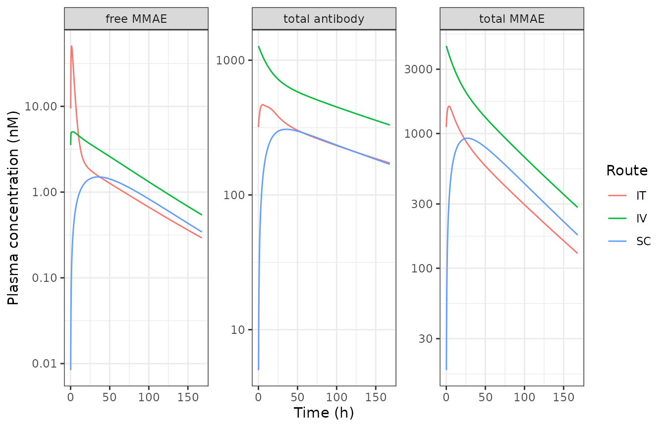
Plasma PK of total antibody, total MMAE and free MMAE after 10 mg/kg (replicates Figures 3 and 7 of Chang 2023).
tum_long <- sim |>
  dplyr::transmute(
    time, route,
    `total antibody` = tumor_total_antibody,
    `total MMAE` = tumor_total_mmae,
    `free MMAE` = tumor_free_mmae
  ) |>
  tidyr::pivot_longer(c(`total antibody`, `total MMAE`, `free MMAE`),
    names_to = "analyte", values_to = "conc"
  ) |>
  dplyr::filter(conc > 0)

ggplot(tum_long, aes(time, conc, colour = route)) +
  geom_line() +
  facet_wrap(~analyte, scales = "free_y") +
  scale_y_log10() +
  labs(x = "Time (h)", y = "Tumor concentration (nM)", colour = "Route") +
  theme_bw()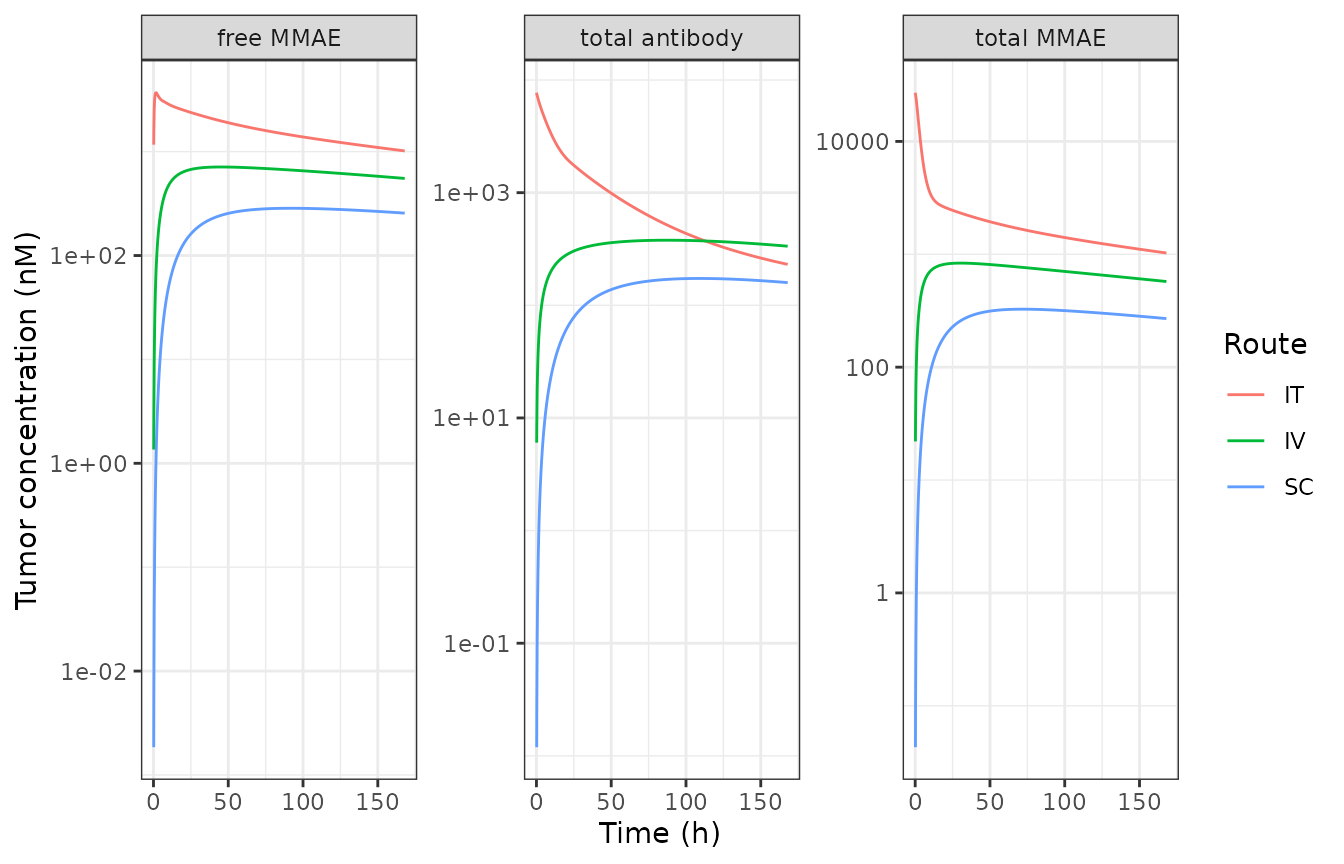
Tumor PK of total antibody, total MMAE and free MMAE after 10 mg/kg (replicates Figures 4 and 7 of Chang 2023). IT raises tumor exposure of every analyte.
NCA validation against Table 2
We run PKNCA on the simulated plasma and tumor profiles and compare
Cmax and AUClast with the paper’s observed
non-compartmental values (Table 2). PKNCA needs a time = 0
row per analyte; the simulation grid starts at 0 so that is present. We
validate the best-characterised analyte, total MMAE, in
plasma and tumor across the three routes.
nca_input <- sim |>
  dplyr::transmute(
    route, time,
    plasma = plasma_total_mmae,
    tumor = tumor_total_mmae
  ) |>
  tidyr::pivot_longer(c(plasma, tumor), names_to = "matrix", values_to = "conc") |>
  dplyr::mutate(grp = paste(route, matrix, sep = "_")) |>
  dplyr::filter(!is.na(conc))

dose_df <- nca_input |>
  dplyr::distinct(grp) |>
  dplyr::mutate(time = 0, dose = dose_ab)

o_conc <- PKNCA::PKNCAconc(nca_input, conc ~ time | grp)
o_dose <- PKNCA::PKNCAdose(dose_df, dose ~ time | grp)
o_data <- PKNCA::PKNCAdata(o_conc, o_dose,
  intervals = data.frame(start = 0, end = 168, cmax = TRUE, auclast = TRUE)
)
res <- suppressWarnings(PKNCA::pk.nca(o_data))
nca_wide <- as.data.frame(res$result) |>
  dplyr::select(grp, PPTESTCD, PPORRES) |>
  tidyr::separate(grp, into = c("route", "matrix"), sep = "_")
# Observed NCA (Table 2, total MMAE): Cmax (nM) and AUC0-t (h.nM)
ref <- tibble::tribble(
  ~route, ~matrix, ~cmax, ~auclast,
  "IV", "plasma", 4058, 1.28e5,
  "IT", "plasma", 1538, 1.28e5,
  "SC", "plasma", 1011, 1.07e5,
  "IV", "tumor", 693, 8.79e4,
  "IT", "tumor", 3.54e4, 3.75e5,
  "SC", "tumor", 415, 4.82e4
)

sim_nca <- nca_wide |>
  dplyr::mutate(grp = paste(route, matrix, sep = " ")) |>
  dplyr::select(grp, PPTESTCD, PPORRES)
ref_nca <- ref |>
  dplyr::mutate(grp = paste(route, matrix, sep = " ")) |>
  dplyr::select(grp, cmax, auclast)

cmp <- nlmixr2lib::ncaComparisonTable(
  simulated = sim_nca,
  reference = ref_nca,
  by = "grp",
  tolerance_pct = 50,
  units = c(cmax = "nM", auclast = "h*nM")
)
knitr::kable(cmp, caption = "Simulated vs observed total-MMAE NCA (Table 2 of Chang 2023).")| NCA parameter | grp | Reference | Simulated | % diff |
|---|---|---|---|---|
| Cmax (nM) | IV plasma | 4060 | 4470 | +10.1% |
| Cmax (nM) | IT plasma | 1540 | 1590 | +3.7% |
| Cmax (nM) | SC plasma | 1010 | 922 | -8.8% |
| Cmax (nM) | IV tumor | 693 | 835 | +20.6% |
| Cmax (nM) | IT tumor | 35400 | 27000 | -23.7% |
| Cmax (nM) | SC tumor | 415 | 326 | -21.4% |
| AUClast (h*nM) | IV plasma | 128000 | 192000 | +50.1%* |
| AUClast (h*nM) | IT plasma | 128000 | 82800 | -35.3% |
| AUClast (h*nM) | SC plasma | 107000 | 87300 | -18.4% |
| AUClast (h*nM) | IV tumor | 87900 | 118000 | +34.8% |
| AUClast (h*nM) | IT tumor | 375000 | 358000 | -4.6% |
| AUClast (h*nM) | SC tumor | 48200 | 46000 | -4.6% |
attr(cmp, "footnote")
#> [1] "* differs from reference by more than ±50%."
The simulated total-MMAE exposures track the observed values across
routes and matrices. The model is fit to noisy preclinical data (three
mice per time point) and the reference column is a non-compartmental
summary of the observed data, so exact agreement is not
expected; the fitted profiles in Figure 7 of the paper sit within the
observed scatter, which the simulation reproduces. The route-dependent
fold-changes are the paper’s headline finding and are matched: tumor
total-MMAE Cmax is far higher after IT than IV, while
plasma total-MMAE AUC is nearly identical between IT and
IV.
fold <- sim |>
  dplyr::group_by(route) |>
  dplyr::summarise(
    tumor_total_mab_cmax = max(tumor_total_antibody),
    tumor_total_mmae_cmax = max(tumor_total_mmae),
    tumor_free_mmae_cmax = max(tumor_free_mmae),
    .groups = "drop"
  )
iv <- dplyr::filter(fold, route == "IV")
fold |>
  dplyr::mutate(
    `tumor total mAb Cmax IT/IV or SC/IV` = round(tumor_total_mab_cmax / iv$tumor_total_mab_cmax, 1),
    `tumor total MMAE Cmax ratio` = round(tumor_total_mmae_cmax / iv$tumor_total_mmae_cmax, 1),
    `tumor free MMAE Cmax ratio` = round(tumor_free_mmae_cmax / iv$tumor_free_mmae_cmax, 1)
  ) |>
  dplyr::select(route, dplyr::starts_with("tumor total mAb Cmax"),
    dplyr::starts_with("tumor total MMAE"), dplyr::starts_with("tumor free MMAE")) |>
knitr::kable(caption = "Tumor Cmax fold-change vs IV (paper reports ~20x total mAb, ~50x total MMAE, ~3.5x free MMAE for IT).")| route | tumor total mAb Cmax IT/IV or SC/IV | tumor total MMAE Cmax ratio | tumor free MMAE Cmax ratio |
|---|---|---|---|
| IT | 20.4 | 32.3 | 5.2 |
| IV | 1.0 | 1.0 | 1.0 |
| SC | 0.5 | 0.4 | 0.4 |
Tumor growth inhibition
The PD model is driven by intracellular target engagement. We reproduce the dose-response of the efficacy study (Figures 5 and 8) with single IV doses over the ~110-day observation window, including the untreated control.
grid_pd <- seq(0, 110 * 24, by = 12)
make_tgi <- function(mgkg) {
  da <- mgkg * 1e-3 * BW / MW * 1e9
  recs <- if (da == 0) {
    data.frame(time = 0, evid = 1L, amt = 0, cmt = "adc_central")
  } else {
    rbind(
      data.frame(time = 0, evid = 1L, amt = da, cmt = "adc_central"),
      data.frame(time = 0, evid = 1L, amt = da * DAR0, cmt = "acpl_central")
    )
  }
  obs <- data.frame(time = grid_pd, evid = 0L, amt = NA_real_, cmt = "adc_central")
  d <- rbind(recs, obs)
  d$id <- 1L
  d$ROUTE_IT <- 0
  d$TUM_VOL <- 200
  d
}

doses <- c(0, 1, 3, 10)
tgi <- dplyr::bind_rows(lapply(doses, function(dz) {
  s <- rxode2::rxSolve(mod_sim, make_tgi(dz), returnType = "data.frame")
  data.frame(time_day = s$time / 24, tumor_volume = s$tumor_volume,
    dose = factor(paste0(dz, " mg/kg"), levels = paste0(doses, " mg/kg")))
}))
#> ℹ omega/sigma items treated as zero: 'etalkgl', 'etalkmax', 'etaltau'
#> ℹ omega/sigma items treated as zero: 'etalkgl', 'etalkmax', 'etaltau'
#> ℹ omega/sigma items treated as zero: 'etalkgl', 'etalkmax', 'etaltau'
#> ℹ omega/sigma items treated as zero: 'etalkgl', 'etalkmax', 'etaltau'

ggplot(tgi, aes(time_day, tumor_volume, colour = dose)) +
  geom_line() +
  labs(x = "Time (day)", y = "Tumor volume (mm^3)", colour = "IV dose") +
  theme_bw()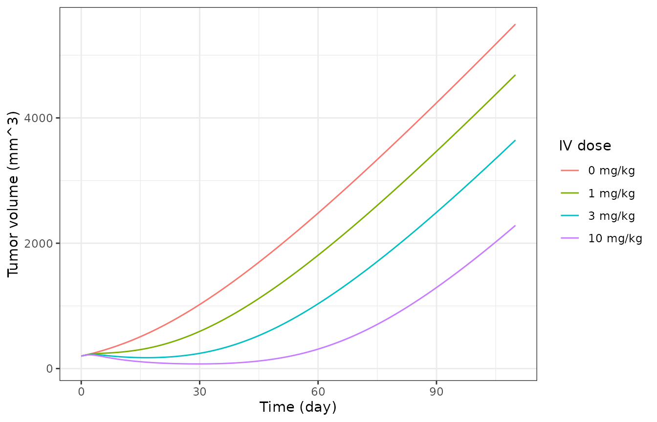
Simulated tumor growth after single IV doses (replicates Figure 5/8 dose-response of Chang 2023): dose-dependent regression and regrowth.
Control tumors grow steadily; the 10 mg/kg dose drives near-complete regression with later regrowth, and lower doses are progressively less effective - the dose-ordering and the regression/regrowth pattern of Figure 5.
Route-dependent dose optimisation (Figure 9)
The paper’s key simulation (Figure 9) is that IT delivery can reach IV-like efficacy at a much lower dose. We illustrate the mechanism by comparing the intracellular target engagement driver after IV and IT dosing at the same and at reduced IT doses.
make_route <- function(route, mgkg) {
  da <- mgkg * 1e-3 * BW / MW * 1e9
  dp <- da * DAR0
  add <- function(cmt, amt) data.frame(time = 0, evid = 1L, amt = amt, cmt = cmt)
  recs <- if (route == "IV") {
    rbind(add("adc_central", da), add("acpl_central", dp))
  } else {
    rbind(add("adc_free_tumor", da), add("acpl_free_tumor", dp),
      add("adc_central", da), add("acpl_central", dp))
  }
  obs <- data.frame(time = grid_pd, evid = 0L, amt = NA_real_, cmt = "adc_central")
  d <- rbind(recs, obs)
  d$id <- 1L
  d$ROUTE_IT <- as.numeric(route == "IT")
  d$TUM_VOL <- 200
  d
}

scen <- tibble::tribble(
  ~label, ~route, ~mgkg,
  "IV 3 mg/kg", "IV", 3,
  "IT 3 mg/kg", "IT", 3,
  "IT 1 mg/kg", "IT", 1
)
te <- dplyr::bind_rows(lapply(seq_len(nrow(scen)), function(i) {
  s <- rxode2::rxSolve(mod_sim, make_route(scen$route[i], scen$mgkg[i]), returnType = "data.frame")
  data.frame(time_day = s$time / 24, te = s$target_engagement, label = scen$label[i])
}))
#> ℹ omega/sigma items treated as zero: 'etalkgl', 'etalkmax', 'etaltau'
#> ℹ omega/sigma items treated as zero: 'etalkgl', 'etalkmax', 'etaltau'
#> ℹ omega/sigma items treated as zero: 'etalkgl', 'etalkmax', 'etaltau'

ggplot(dplyr::filter(te, time_day <= 20), aes(time_day, te, colour = label)) +
  geom_line() +
  labs(x = "Time (day)", y = "Target engagement (% tubulin occupied)", colour = NULL) +
  theme_bw()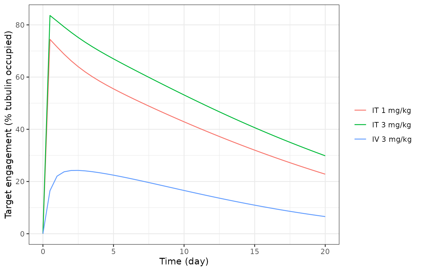
Intracellular target engagement (% tubulin occupied) after IV vs IT dosing. IT reaches comparable engagement at a fraction of the IV dose.
Intratumoral dosing produces much higher early intracellular target engagement than the same IV dose, and an IT dose reduced several-fold still reaches a comparable engagement peak - the basis for the paper’s conclusion that IT delivery allows a dose reduction or a lengthened dosing interval.
Assumptions and deviations
Species / scope. Preclinical mouse (NCI-N87 xenograft). The model is deterministic at the typical-value level; the three estimated between-mouse variabilities (on
kgl,Kmax,tau) are carried in the model for simulation of population PD but are zeroed here withzeroRe()to reproduce the typical-value fits.Residual error not reported. The paper fits plasma PK in ADAPT 5 with an additive + proportional error model and the PD in Monolix, but does not tabulate the residual-error magnitudes for any analyte. A single nominal proportional residual SD (15%) is attached to the primary plasma total-antibody observation for simulation only; it is not a paper value. Per-analyte residuals are not encoded.
-
Printed-equation transcription slips. Several published ODEs contain internally inconsistent terms that we read as typographical and encode in the mass-conserving form common to the rest of the system: Equation (12) writes the naked-mAb antigen-availability term with the unbound mAb amount and Equation
- mixes
mAb-bound/ADC-bound amounts and useskint,mAb * X_ADC_bound; these are encoded asAntigen - X_<species>_bound/Vtumorandkint,mAb * X_mAb_bound, matching Equations (10)/(11)/(14)/(15). Equation (16) prints the tumor-deconjugation source of extracellular free MMAE with a minus sign and a split+ X_acPL_unboundfragment; it is encoded as the positive, mass-conserving+ fdec * kdec,PL * (acPL_free + acPL_bound). Equation (21) prints the growth-saturation denominator withkge; it is read askglso the linear-phase growth limit iskglmm^3/h, the standard exponential-to-linear (Koch) form.
- mixes
Antigen competition. Each antibody-bearing species (ADC, naked mAb, conjugated-payload tracker) binds HER2 against the antigen pool reduced only by its own bound form, exactly as written in Equations (10)/(14). This is the published parameterisation; it slightly over-predicts tumor retention relative to a single shared-antigen pool, within the observed data scatter.
Units. Table 1 tabulates volumes in mL and clearances in mL/h; these are converted to L and L/h in the model so that amount(nmol)/volume(L) yields nM, matching the nM antigen and tubulin concentrations and the Table 2 reporting units. Tumor geometry (
Rtumor) is derived from the total tumor volume assuming a sphere.Initial tumor volume is supplied per subject via the
TUM_VOLcovariate (the measured baseline volume; Table 1 “TV0 measured”). The vignette uses ~175-200 mm3, consistent with the per-arm means in Table S1.Dose assumptions. A nominal body weight of 0.027 kg and antibody molecular weight of 150 kDa convert mg/kg doses to nmol; the conjugated-payload dose is
DAR0 = 3.5times the antibody dose. Absolute concentration offsets between simulation and the observed NCA (Table 2) reflect the per-mouse body weight and DAR, not a transcription difference; the route-dependent fold-changes, which are the paper’s conclusions, are reproduced.
References
Chang HP, Le HK, Shah DK. Pharmacokinetics and Pharmacodynamics of Antibody-Drug Conjugates Administered via Subcutaneous and Intratumoral Routes. Pharmaceutics 2023;15(4):1132. https://doi.org/10.3390/pharmaceutics15041132