5-Fluorouracil and leukocyte myelosuppression (Arshad 2020)
Source:vignettes/articles/Arshad_2020_fluorouracil.Rmd
Arshad_2020_fluorouracil.RmdModel and source
- Citation: Arshad U, Ploylearmsaeng SA, Karlsson MO, Doroshyenko O, Langer D, Schomig E, Kunze S, Guner SA, Skripnichenko R, Ullah S, Jaehde U, Fuhr U, Jetter A, Taubert M. Prediction of exposure-driven myelotoxicity of continuous infusion 5-fluorouracil by a semi-physiological pharmacokinetic-pharmacodynamic model in gastrointestinal cancer patients. Cancer Chemother Pharmacol. 2020;85(4):711-722. doi:10.1007/s00280-019-04028-5
- Description: Semi-physiological PK/PD model of continuous-infusion 5-fluorouracil (5-FU) in adults with gastrointestinal cancer (Arshad 2020). 5-FU follows a two-compartment model with linear elimination; a fixed 85% of 5-FU clearance forms 5-fluoro-5,6-dihydrouracil (5FUH2), which follows a one-compartment model. A single linear body-surface-area effect is shared by the 5-FU and 5FUH2 clearances. 5-FU plasma concentration drives a Friberg-style leukocyte myelosuppression chain (proliferating pool, three transit compartments, circulating cells, feedback exponent fixed at 0.17) through a linear drug effect whose slope differs between 5-FU monotherapy and 5-FU plus cisplatin.
- Article: https://doi.org/10.1007/s00280-019-04028-5 (open access; PMC7125253)
Arshad et al. gave 30 patients with gastrointestinal cancer 5-FU 650 or 1000 mg/m^2/day as a 5-day continuous intravenous infusion. The 14 patients with oesophageal cancer also received cisplatin 20 mg/m^2/day. Plasma 5-FU, its first catabolite 5-fluoro-5,6-dihydrouracil (5FUH2) and total white blood cell (WBC) counts were fitted simultaneously in NONMEM. 5-FU follows a two-compartment model. A fixed 85% of 5-FU clearance forms 5FUH2, which follows a one-compartment model. A single linear body-surface-area (BSA) effect scales both clearances. The 5-FU concentration drives a Friberg myelosuppression chain through a linear drug effect. The slope of that effect is larger in patients who also received cisplatin.
No supplement or erratum was found for this article (literature check, 2026-09-25).
Population
str(rxode2::rxode(readModelDb("Arshad_2020_fluorouracil"))$population)
#> ℹ parameter labels from comments will be replaced by 'label()'
#> List of 13
#>  $ species       : chr "human"
#>  $ n_subjects    : int 30
#>  $ n_studies     : int 1
#>  $ age_range     : chr "37-73 years (median 59.5)"
#>  $ weight_range  : chr "46-111 kg (median 76)"
#>  $ bsa_range     : chr "1.48-2.33 m^2 (median 1.95)"
#>  $ sex_female_pct: num 16.7
#>  $ race_ethnicity: chr "Not reported (single German centre)"
#>  $ disease_state : chr "Gastrointestinal cancer: oesophageal (n = 14, 5-FU + cisplatin) and colorectal / rectal / anal (n = 16, 5-FU + "| __truncated__
#>  $ dose_range    : chr "5-FU 650 or 1000 mg/m^2/day as a 5-day continuous IV infusion (first cycle only); cisplatin 20 mg/m^2/day for 5"| __truncated__
#>  $ regions       : chr "Germany (University Hospital Cologne, 2002-2005)"
#>  $ baseline_wbc  : chr "Median 6.90 x 10^9/L (range 4.68-11.28)"
#>  $ notes         : chr "199 5-FU and 251 5FUH2 plasma concentrations; 135 total WBC counts from 29 patients. Estimation with FOCE-I in "| __truncated__
Thirty patients (25 men, 5 women) aged 37-73 years (median 59.5) completed the first cycle (Table 1). Median body weight was 76 kg (46-111) and median BSA was 1.95 m^2 (1.48-2.33). Median baseline WBC count was 6.90 x 10^9/L. Sixteen patients with colorectal, rectal or anal cancer received 5-FU with radiotherapy. Fourteen with oesophageal cancer received 5-FU plus cisplatin. The analysis used 199 5-FU and 251 5FUH2 concentrations and 135 WBC counts from 29 patients.
Source trace
| Model element | Value | Source |
|---|---|---|
lcl (CL5FU at BSA 1.95 m^2) |
249 L/h | Table 3, bootstrap column (NONMEM 256) |
lvc (VC,5FU) |
5.56 L | Table 3, bootstrap (NONMEM 5.85) |
lvp (VP,5FU) |
28.5 L | Table 3, bootstrap (NONMEM 24.0) |
lq (Q) |
14.8 L/h | Table 3, bootstrap (NONMEM 17.3) |
e_bsa_cl (shared by CL5FU and CL5FUH2) |
0.77 per m^2 | Table 3, footnote a; Abstract “77%/m2”; Results (single shared parameter) |
fm |
0.85 (fixed) | Methods, Pharmacokinetic analysis; Table 3 |
lcl_5fuh2 |
121 L/h | Table 3, bootstrap (NONMEM 124) |
lvc_5fuh2 |
96.7 L | Table 3, bootstrap (NONMEM 100) |
lcirc0 |
6.86 x 10^9/L | Table 3, bootstrap (NONMEM 7.16) |
lmtt |
281 h | Table 3, bootstrap (NONMEM 261) |
lslope_mono |
1.17 L/mg | Table 3, bootstrap (NONMEM 1.31) |
lslope_comb |
2.82 L/mg | Table 3, bootstrap (NONMEM 2.10) |
gamma |
0.17 (fixed) | Results, Pharmacodynamic model; Table 3 |
| IIV CL5FU, VC,5FU, CL5FUH2, VC,5FUH2, CIRC0 | 23.0, 145, 28.9, 59.6, 16.4 %CV | Table 3, bootstrap; omega^2 = log(CV^2 + 1)
|
| Proportional RUV 5-FU, 5FUH2, WBC | sigma^2 0.32, 0.14, 0.08 | Table 3 (“RUV (sigma2)”); SD = sqrt |
| Two-compartment 5-FU, one-compartment 5FUH2 | – | Results, Pharmacokinetic model; Fig. 1 |
5FUH2 formation fm * CL5FU
|
– | Fig. 1 (CL5FU x Fm) |
BSA form CL = TVCL * (1 + 0.77 * (BSA - 1.95))
|
– | Table 3 footnote a; Table 1 median BSA |
Friberg chain, three transits, kprol = ktr = kcirc,
MTT = 4/ktr
|
– | Methods, Pharmacodynamic analysis; Fig. 1 |
Feedback (Circ0/Circ)^gamma, effect
kprol * (1 - slope * Cp)
|
– | Methods, Pharmacodynamic analysis |
| Slope by cisplatin group | – | Results, Covariate relationships; Table 3 |
Which column of Table 3?
Table 3 prints two sets of estimates: the NONMEM estimates and the bootstrap medians. They differ by up to 34% (Slopecomb 2.10 vs 2.82 L/mg). The Abstract and Discussion quote the bootstrap medians throughout (249 L/h, 5.56 L, 28.5 L, 121 L/h, 96.7 L, 6.86 x 10^9/L, 281 h, 2.82 and 1.17 L/mg, 77%/m^2).
The paper’s own simulation settles which set the authors used. Figure 3 (left panel) shows a typical patient on a 5-day infusion, with WBC nadirs of 4.29 x 10^9/L without cisplatin and 2.26 x 10^9/L with it. The curves start at 6.86 x 10^9/L, which is the bootstrap CIRC0 (the NONMEM CIRC0 is 7.16). The figure does not state the dose. So for each column, the chunk below finds the daily dose that gives the monotherapy nadir of 4.29. It then predicts the combination nadir at that same dose. Both arms share every parameter except the slope, so only a column whose slope ratio is right can hit both nadirs.
mod <- readModelDb("Arshad_2020_fluorouracil")
ui <- rxode2::rxode(mod)
#> ℹ parameter labels from comments will be replaced by 'label()'

nonmem_ui <- ui |>
  rxode2::ini(
    lcl = log(256), lvc = log(5.85), lvp = log(24.0), lq = log(17.3),
    e_bsa_cl = 0.71, lcl_5fuh2 = log(124), lvc_5fuh2 = log(100),
    lcirc0 = log(7.16), lmtt = log(261),
    lslope_mono = log(1.31), lslope_comb = log(2.10)
  )
#> ℹ change initial estimate of `lcl` to `5.54517744447956`
#> ℹ change initial estimate of `lvc` to `1.76644166124377`
#> ℹ change initial estimate of `lvp` to `3.17805383034795`
#> ℹ change initial estimate of `lq` to `2.85070650150373`
#> ℹ change initial estimate of `e_bsa_cl` to `0.71`
#> ℹ change initial estimate of `lcl_5fuh2` to `4.82028156560504`
#> ℹ change initial estimate of `lvc_5fuh2` to `4.60517018598809`
#> ℹ change initial estimate of `lcirc0` to `1.96850998097255`
#> ℹ change initial estimate of `lmtt` to `5.56452040732269`
#> ℹ change initial estimate of `lslope_mono` to `0.27002713721306`
#> ℹ change initial estimate of `lslope_comb` to `0.741937344729377`

typical_wbc <- function(model, events) {
  rxode2::rxSolve(model, events, omega = NA, sigma = NA, returnType = "data.frame")
}

five_day_events <- function(daily_mg, cisplatin, end_day = 60) {
  obs_t <- seq(0, end_day * 24, by = 2)
  dplyr::bind_rows(
    data.frame(
      id = 1L, time = 0, amt = daily_mg * 5, rate = daily_mg / 24, evid = 1L,
      cmt = "central", dvid = NA_integer_
    ),
    data.frame(
      id = 1L, time = obs_t, amt = 0, rate = 0, evid = 0L,
      cmt = NA_character_, dvid = 1L
    )
  ) |>
    dplyr::mutate(BSA = 1.95, CONMED_CISPLATIN = cisplatin) |>
    dplyr::arrange(time, dplyr::desc(evid))
}

nadir_of <- function(model, daily_mg, cisplatin) {
  s <- typical_wbc(model, five_day_events(daily_mg, cisplatin))
  i <- which.min(s$WBC)
  c(nadir = s$WBC[i], tnadir_day = s$time[i] / 24)
}

matched <- lapply(list(bootstrap = ui, nonmem = nonmem_ui), function(m) {
  dose <- uniroot(
    function(d) nadir_of(m, d, 0)[["nadir"]] - 4.29,
    interval = c(500, 5000), tol = 0.5
  )$root
  mono <- nadir_of(m, dose, 0)
  comb <- nadir_of(m, dose, 1)
  data.frame(
    daily_dose = dose, nadir_mono = mono[["nadir"]], nadir_comb = comb[["nadir"]],
    tnadir_mono = mono[["tnadir_day"]], tnadir_comb = comb[["tnadir_day"]]
  )
})
disc <- dplyr::bind_rows(matched, .id = "column") |>
  dplyr::mutate(comb_pct_diff = 100 * (nadir_comb - 2.26) / 2.26)

disc |>
  dplyr::mutate(dplyr::across(-column, \(x) signif(x, 3))) |>
  dplyr::rename(
    "Table 3 column" = column,
    "Daily dose matching mono nadir (mg/day)" = daily_dose,
    "Mono nadir (10^9/L)" = nadir_mono,
    "Comb nadir (10^9/L)" = nadir_comb,
    "Mono Tnadir (day)" = tnadir_mono,
    "Comb Tnadir (day)" = tnadir_comb,
    "Comb nadir vs published 2.26 (%)" = comb_pct_diff
  ) |>
knitr::kable(caption = "Typical patient (BSA 1.95 m^2), 5-day infusion. Published Figure 3: nadirs 4.29 (mono) and 2.26 (comb), Tnadir day 22-25.")| Table 3 column | Daily dose matching mono nadir (mg/day) | Mono nadir (10^9/L) | Comb nadir (10^9/L) | Mono Tnadir (day) | Comb Tnadir (day) | Comb nadir vs published 2.26 (%) |
|---|---|---|---|---|---|---|
| bootstrap | 1760 | 4.29 | 2.26 | 23.0 | 24.2 | 0.0821 |
| nonmem | 1650 | 4.29 | 3.17 | 21.7 | 22.1 | 40.4000 |
boot_row <- disc[disc$column == "bootstrap", ]
nonmem_row <- disc[disc$column == "nonmem", ]
stopifnot(
  # Deterministic typical-value solves: tight bounds are appropriate.
  abs(boot_row$comb_pct_diff) < 5,
  abs(nonmem_row$comb_pct_diff) > 15,
  boot_row$tnadir_mono >= 22, boot_row$tnadir_comb <= 25
)
With the bootstrap column, the dose that gives the 4.29 monotherapy
nadir (about 1750 mg/day, or about 900 mg/m^2/day at 1.95 m^2) also
gives the published combination nadir to within 1%. The nadirs fall on
days 23-24, within the day 22-25 range stated in the Discussion. The
NONMEM column cannot hit both nadirs at any single dose. The packaged
model therefore uses the bootstrap medians, and each ini()
comment also gives the NONMEM estimate.
Replicate Figure 3
fig3l <- dplyr::bind_rows(
  typical_wbc(mod, five_day_events(boot_row$daily_dose, 0, 50)) |>
    dplyr::mutate(arm = "5FU mono"),
  typical_wbc(mod, five_day_events(boot_row$daily_dose, 1, 50)) |>
    dplyr::mutate(arm = "5FU + cisplatin")
)
#> ℹ parameter labels from comments will be replaced by 'label()'
ggplot(fig3l, aes(time / 24, WBC, linetype = arm)) +
  geom_line() +
  coord_cartesian(ylim = c(0, 8)) +
  labs(
    x = "Time after start of infusion (days)", y = "Total WBC count (10^9/L)",
    linetype = NULL,
    caption = sprintf("Replicates Figure 3 (left) of Arshad 2020; 5-day infusion of %.0f mg/day.", boot_row$daily_dose)
  ) +
  theme_bw()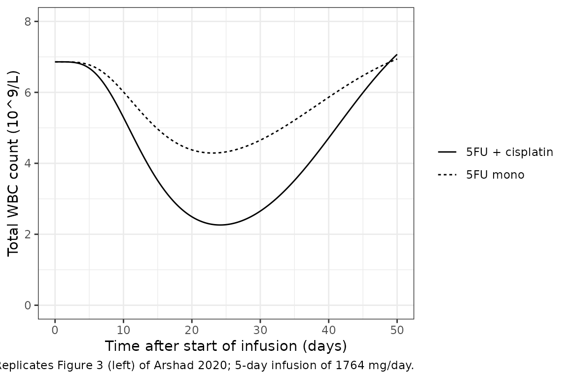
The right panel of Figure 3 compares the 5-FU component of one FOLFIRINOX course (400 mg/m^2 bolus, then 2400 mg/m^2 over 46 h) with one de Gramont day (300 mg/m^2 bolus, then 300 mg/m^2 over 24 h). The chunk below simulates both regimens at BSA 1.95 m^2 with each slope.
regimen_events <- function(bolus, infused, dur, cisplatin, bsa = 1.95) {
  obs_t <- seq(0, 100 * 24, by = 4)
  dplyr::bind_rows(
    data.frame(time = 0, amt = bolus * bsa, rate = 0, evid = 1L, cmt = "central", dvid = NA_integer_),
    data.frame(time = 0, amt = infused * bsa, rate = infused * bsa / dur, evid = 1L, cmt = "central", dvid = NA_integer_),
    data.frame(time = obs_t, amt = 0, rate = 0, evid = 0L, cmt = NA_character_, dvid = 1L)
  ) |>
    dplyr::mutate(id = 1L, BSA = bsa, CONMED_CISPLATIN = cisplatin) |>
    dplyr::arrange(time, dplyr::desc(evid))
}
regimens <- tidyr::expand_grid(
  regimen = c("FOLFIRINOX", "de Gramont"), cisplatin = c(0, 1)
) |>
  dplyr::mutate(
    bolus = ifelse(regimen == "FOLFIRINOX", 400, 300),
    infused = ifelse(regimen == "FOLFIRINOX", 2400, 300),
    dur = ifelse(regimen == "FOLFIRINOX", 46, 24)
  )
fig3r <- dplyr::bind_rows(lapply(seq_len(nrow(regimens)), function(i) {
  r <- regimens[i, ]
  typical_wbc(mod, regimen_events(r$bolus, r$infused, r$dur, r$cisplatin)) |>
    dplyr::mutate(
      regimen = r$regimen,
      slope = ifelse(r$cisplatin == 1, "Slope comb", "Slope mono")
    )
}))
fig3r |>
  dplyr::group_by(regimen, slope) |>
  dplyr::summarise(nadir = min(WBC), tnadir_day = time[which.min(WBC)] / 24, .groups = "drop") |>
  dplyr::mutate(published = ifelse(regimen == "FOLFIRINOX", 1.06, 4.20)) |>
  dplyr::mutate(dplyr::across(c(nadir, tnadir_day), \(x) signif(x, 3))) |>
  dplyr::rename(
    "Regimen" = regimen, "Slope used" = slope, "Simulated nadir (10^9/L)" = nadir,
    "Simulated Tnadir (day)" = tnadir_day, "Published nadir (10^9/L)" = published
  ) |>
knitr::kable(caption = "Figure 3 (right panel) regimens, typical patient, BSA 1.95 m^2.")| Regimen | Slope used | Simulated nadir (10^9/L) | Simulated Tnadir (day) | Published nadir (10^9/L) |
|---|---|---|---|---|
| FOLFIRINOX | Slope comb | 3.41 | 21.8 | 1.06 |
| FOLFIRINOX | Slope mono | 5.11 | 21.0 | 1.06 |
| de Gramont | Slope comb | 5.89 | 20.3 | 4.20 |
| de Gramont | Slope mono | 6.44 | 20.2 | 4.20 |
ggplot(fig3r, aes(time / 24, WBC, linetype = regimen)) +
  geom_line() +
  facet_wrap(~slope) +
  labs(
    x = "Time after start of infusion (days)", y = "Total WBC count (10^9/L)",
    linetype = NULL, caption = "Compare Figure 3 (right) of Arshad 2020."
  ) +
  theme_bw()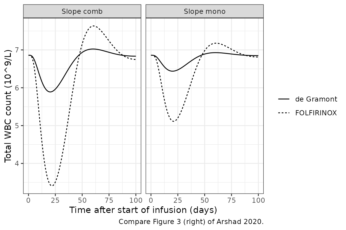
The right panel cannot be reproduced from the printed information. The paper shows nadirs of 1.06 (FOLFIRINOX) and 4.20 (de Gramont) x 10^9/L, and a rebound to about 9 x 10^9/L. The model gives much shallower nadirs with either slope. A FOLFIRINOX course delivers about 60% of the 5-FU AUC of the left-panel 5-day infusion, yet the paper shows a deeper nadir for it than the left panel’s combination nadir. So the right panel must have used settings the paper does not report, such as a different dose basis, BSA or number of administrations. The left panel, which the text describes in full, is reproduced. The parameters are not tuned to the right panel.
Virtual cohort
The cohort has two arms, 5-FU alone and 5-FU plus cisplatin, with 100 virtual patients each. BSA is drawn from a normal distribution with mean 1.95 m^2 and SD 0.2, truncated to the observed 1.48-2.33 m^2 (Table 1). The paper does not report how many patients received 650 vs 1000 mg/m^2/day, so each virtual patient gets one of the two doses with equal probability.
set.seed(20200309)
rxode2::rxSetSeed(20200309)
n_per_arm <- 100
cohort <- tibble::tibble(
  id = seq_len(2 * n_per_arm),
  CONMED_CISPLATIN = rep(c(0, 1), each = n_per_arm),
  BSA = pmin(pmax(rnorm(2 * n_per_arm, 1.95, 0.2), 1.48), 2.33),
  dose_m2 = sample(c(650, 1000), 2 * n_per_arm, replace = TRUE)
) |>
  dplyr::mutate(
    daily_mg = dose_m2 * BSA,
    treatment = ifelse(CONMED_CISPLATIN == 1, "5FU + cisplatin", "5FU mono")
  )

obs_times <- sort(unique(c(
  seq(0, 24, by = 0.5), seq(24, 120, by = 4), 120 + c(5, 30, 60, 90) / 60,
  seq(124, 60 * 24, by = 12)
)))
ev_cohort <- dplyr::bind_rows(
  cohort |>
    dplyr::mutate(
      time = 0, amt = daily_mg * 5, rate = daily_mg / 24, evid = 1L,
      cmt = "central", dvid = NA_integer_
    ),
  tidyr::expand_grid(cohort, time = obs_times) |>
    dplyr::mutate(amt = 0, rate = 0, evid = 0L, cmt = NA_character_, dvid = 1L)
) |>
  dplyr::arrange(id, time, dplyr::desc(evid))

sim <- rxode2::rxSolve(
  mod, ev_cohort,
  sigma = NA, returnType = "data.frame",
  keep = c("treatment", "dose_m2", "BSA")
)
Simulated profiles (compare Figure 2)
Figure 2 of the paper is a visual predictive check of 5-FU, 5FUH2 and WBC. The bands below are the 5th, 50th and 95th percentiles of the individual predictions of the virtual cohort (residual error not added).
long <- sim |>
  dplyr::select(id, time, treatment, Cc, Cc_5fuh2, WBC) |>
  tidyr::pivot_longer(c(Cc, Cc_5fuh2, WBC), names_to = "output", values_to = "value") |>
  dplyr::mutate(output = dplyr::recode(
    output,
    Cc = "5-FU (mg/L)", Cc_5fuh2 = "5FUH2 (mg/L)", WBC = "WBC (10^9/L)"
  ))
bands <- long |>
  dplyr::filter(output == "WBC (10^9/L)" | time <= 130) |>
  dplyr::group_by(output, treatment, time) |>
  dplyr::summarise(
    p05 = quantile(value, 0.05), p50 = median(value), p95 = quantile(value, 0.95),
    .groups = "drop"
  )
ggplot(bands, aes(time / 24, p50, colour = treatment, fill = treatment)) +
  geom_ribbon(aes(ymin = p05, ymax = p95), alpha = 0.15, colour = NA) +
  geom_line() +
  facet_wrap(~output, scales = "free", ncol = 1) +
  labs(
    x = "Time after start of infusion (days)", y = NULL, colour = NULL, fill = NULL,
    caption = "Median and 90% interval of individual predictions; compare Figure 2 of Arshad 2020."
  ) +
  theme_bw()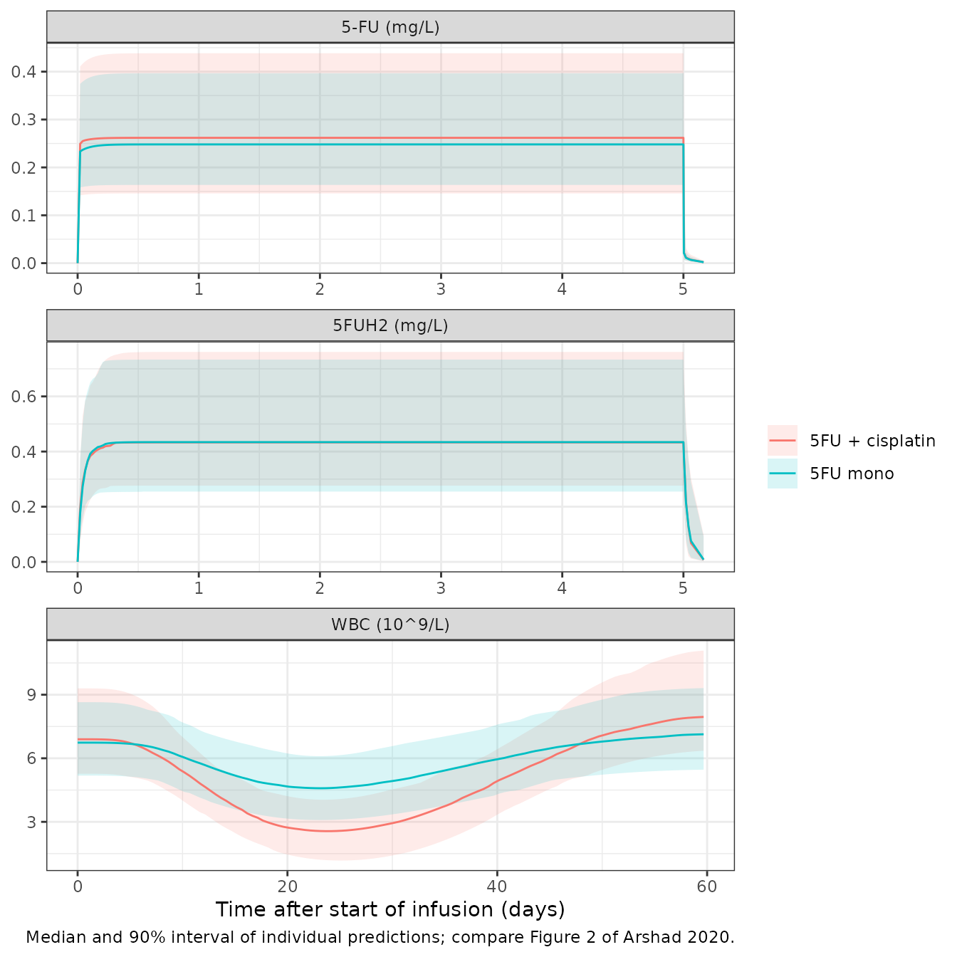
PKNCA validation
Table 3 reports the median AUC over 24 h of infusion: 6.72 mg h/L for 5-FU and 12.2 mg h/L for 5FUH2. Both values pool the 650 and 1000 mg/m^2/day patients. The footnote says this AUC came from an extra integrating compartment in NONMEM, but it does not say which 24 h. Both species reach steady state within a few hours of the start of the infusion, apart from patients with a very large 5FUH2 volume. PKNCA therefore computes the 24-48 h AUC, a steady-state dosing day, for each virtual patient.
conc <- sim |>
  dplyr::filter(time <= 48) |>
  dplyr::select(id, time, treatment, Cc, Cc_5fuh2) |>
  tidyr::pivot_longer(c(Cc, Cc_5fuh2), names_to = "analyte", values_to = "conc") |>
  dplyr::filter(!is.na(conc)) |>
  dplyr::mutate(analyte = ifelse(analyte == "Cc", "5FU", "5FUH2"))
dose_df <- tidyr::expand_grid(
  cohort |> dplyr::select(id, treatment, daily_mg),
  analyte = c("5FU", "5FUH2")
) |>
  dplyr::mutate(time = 0, amt = daily_mg * 5, duration = 120)

conc_obj <- PKNCA::PKNCAconc(conc, conc ~ time | treatment + analyte + id)
dose_obj <- PKNCA::PKNCAdose(dose_df, amt ~ time | treatment + analyte + id, duration = "duration")
intervals <- data.frame(start = 24, end = 48, auclast = TRUE)
nca_res <- PKNCA::pk.nca(PKNCA::PKNCAdata(conc_obj, dose_obj, intervals = intervals))

nca_tbl <- as.data.frame(nca_res) |>
  dplyr::filter(PPTESTCD == "auclast") |>
  dplyr::group_by(analyte) |>
  dplyr::summarise(
    median = median(PPORRES), p05 = quantile(PPORRES, 0.05), p95 = quantile(PPORRES, 0.95),
    .groups = "drop"
  )
nca_tbl |>
  dplyr::mutate(dplyr::across(-analyte, \(x) signif(x, 3))) |>
  dplyr::rename(
    "Analyte" = analyte, "Median AUC24-48 (mg h/L)" = median,
    "5th percentile" = p05, "95th percentile" = p95
  ) |>
knitr::kable(caption = "PKNCA AUC over the second infusion day (24-48 h), both arms pooled.")| Analyte | Median AUC24-48 (mg h/L) | 5th percentile | 95th percentile |
|---|---|---|---|
| 5FU | 6.17 | 3.84 | 10.2 |
| 5FUH2 | 10.40 | 6.21 | 18.3 |
Comparison against published values
published_nca <- tibble::tibble(
  analyte = c("5FU", "5FUH2"),
  auclast = c(6.72, 12.2)
)
cmp <- nlmixr2lib::ncaComparisonTable(
  simulated = nca_res,
  reference = published_nca,
  by = "analyte",
  params = "auclast",
  units = c(auclast = "mg*h/L"),
  tolerance_pct = 20
)
knitr::kable(cmp, caption = "Simulated median AUC24-48 vs Table 3 of Arshad 2020. * differs from reference by >20%.")| NCA parameter | analyte | Reference | Simulated | % diff |
|---|---|---|---|---|
| AUClast (mg*h/L) | 5FU | 6.72 | 6.17 | -8.2% |
| AUClast (mg*h/L) | 5FUH2 | 12.2 | 10.4 | -14.6% |
The simulated 5-FU AUC depends on the unreported split between the
650 and 1000 mg/m^2/day patients. The ratio of 5FUH2 to 5-FU AUC does
not. With a mass basis it equals fm * CL5FU / CL5FUH2 for
each patient, and the BSA effect cancels because both clearances share
it. For the typical patient that is 0.85 x 249 / 121 = 1.75, against
12.2 / 6.72 = 1.82 from the Table 3 medians.
ratio <- as.data.frame(nca_res) |>
  dplyr::filter(PPTESTCD == "auclast") |>
  dplyr::select(id, analyte, PPORRES) |>
  tidyr::pivot_wider(names_from = analyte, values_from = PPORRES) |>
  dplyr::mutate(ratio = `5FUH2` / `5FU`)
published_ratio <- 12.2 / 6.72
ratio_summary <- c(
  simulated_median = median(ratio$ratio),
  typical_closed_form = 0.85 * 249 / 121,
  published_median_ratio = published_ratio
)
signif(ratio_summary, 3)
#>       simulated_median    typical_closed_form published_median_ratio
#>                   1.66                   1.75                   1.82
stopifnot(
  # Deterministic: the typical steady-state ratio against the published one.
  abs(ratio_summary[["typical_closed_form"]] / published_ratio - 1) < 0.05,
  # Cohort centre: the median of exp(etalcl - etalcl_5fuh2) is 1, and its
  # sampling SE with 200 patients is about 3%, so 15% is a wide envelope.
  abs(median(ratio$ratio) / ratio_summary[["typical_closed_form"]] - 1) < 0.15
)
The typical ratio is 4% below the ratio of the two published medians. The cohort median lies a few percent lower again, because of the random draws of the two clearance etas. The two Table 3 AUC medians are taken separately over patients, so their quotient is only an approximate reference.
Assumptions and deviations
-
Bootstrap medians, not NONMEM estimates. Table 3
prints both. The packaged values are the bootstrap medians. These are
the values the Abstract and Discussion quote, and they reproduce the
Figure 3 simulation (see “Which column of Table 3?”). The NONMEM
estimates are recorded in the
ini()comments. -
IIV scale. Table 3 reports IIV as %CV without
stating the conversion. The model uses
omega^2 = log(CV^2 + 1). Withomega = CVinstead, the 145% CV on VC,5FU would give omega^2 = 2.10 rather than 1.13. This affects the width of the peak-concentration spread only, not the typical values. -
Residual error scale. The Table 3 header says “RUV
(sigma2)”, so the values are variances and the model uses their square
roots. The NONMEM RSEs (10.2%, 8.06% and 8.70%) are close to the
sqrt(2/N)expected for a variance estimated from 199, 251 and 135 observations. That is consistent with this reading. -
5FUH2 on a mass basis. The paper says PK parameters
used the absolute dose and gives no molecular-weight correction. The
model feeds
fm * CL5FU * Cc(mg) directly into the 5FUH2 compartment. The molar-mass ratio of 5FUH2 to 5-FU is 1.015, so a molar reading would change 5FUH2 concentrations by 1.5%. -
Shared BSA effect. The paper estimated a single BSA
coefficient for both clearances. It is encoded as one parameter,
e_bsa_cl, used in both equations. The BSA formula is not reported. -
Cisplatin indicator. The paper estimated one slope
per group. Here
CONMED_CISPLATINselects between them. In the study the cisplatin group is also the oesophageal-cancer group, so the indicator cannot separate a cisplatin effect from a tumour-site effect. - Dose split in the virtual cohort. The number of patients on 650 vs 1000 mg/m^2/day is not reported, so the virtual cohort assigns them with equal probability.
- Figure 3 right panel is not reproducible from the stated regimens (see above), and the parameters were not adjusted towards it.
- DPYD, TS and MTHFR genotypes were tested but not retained in the final model (Results, Covariate relationships). They are not included.