Model and source
- Citation: Li X-l, Huang S-q, Xiao T, Wang X-p, Kong W, Liu S-j, Zhang Z, Yang Y, Huang S-s, Ni X-j, Lu H-y, Zhang M, Wen Y-g, Shang D-w. Pharmacokinetics of immediate and sustained-release formulations of paroxetine: Population pharmacokinetic approach to guide paroxetine personalized therapy in Chinese psychotic patients. Front Pharmacol. 2022;13:966622. doi:10.3389/fphar.2022.966622
- Description: One-compartment population PK model with first-order absorption for oral paroxetine immediate-release and sustained-release tablets in Chinese psychiatric inpatients receiving therapeutic drug monitoring, with daily dose on CL/F, formulation on V/F and sex on relative bioavailability (Li 2022).
- Article (open access): https://doi.org/10.3389/fphar.2022.966622
Population
Li 2022 analysed retrospective therapeutic-drug-monitoring (TDM) data from psychiatric inpatients treated with paroxetine at the Affiliated Brain Hospital of Guangzhou Medical University, China, between January 2019 and May 2021. The analysis set held 184 patients (103 female, 56%; 81 male) and 372 serum paroxetine concentrations (median 60.55 ng/mL, range 2.62-447.87). Median age was 37.5 years (range 15-90), median body weight 60 kg (printed range 58-96), and median height 164.5 cm (Li 2022 Table 1). Daily doses ranged from 20 to 75 mg and were adjusted during treatment; 85.5% of the concentrations were on immediate-release tablets and 14.5% on 25 mg sustained-release tablets. Samples were drawn 10-22.5 h after the most recent dose, so the data are essentially troughs. Co-medications included olanzapine (16.8%), tandospirone (14.1%), risperidone (13.0%) and metoprolol (5.4%); none was retained as a covariate, and CYP2D6 genotype was not retained either.
The same information is available programmatically via
readModelDb("Li_2022_paroxetine")()$population.
Source trace
Li 2022 gives the final model as four printed equations (Section 3.2.1):
CL/F (L/h) = 21.2 * (dose/40)^-1.03V/F (L) = 8850 * (1 - 0.666 * formulation)Ka (1/h) = 0.908F1 = 1 + (0.475 * SEX)
with formulation = 1 for the immediate-release tablet
and SEX = 1 for female (Methods 2.3.2).
| Equation / parameter | Value | Source location |
|---|---|---|
lka |
fixed(log(0.908)) |
Table 2 ‘Ka (1/h) 0.908 fixed’; Methods 2.3.1 (literature value) |
lcl |
log(21.2) |
Table 2 ‘CL/F (L/h) 21.2’ (RSE 7.2%) |
lvc |
log(8850) |
Table 2 ‘V/F (L) 8,850’ (RSE 17.2%) |
e_dose_cl |
-1.03 |
Table 2 ‘theta CL-dosage’ (RSE 5.7%); Section 3.2.1 CL/F equation, reference 40 mg/day |
e_form_ir_vc |
0.666 |
Table 2 ‘theta V-formulation’ (RSE 9.7%); Section 3.2.1 V/F equation |
e_sexf_fdepot |
0.475 |
Table 2 ‘theta F-sex’ (RSE 25.3%); Section 3.2.1 F1 equation |
etalcl |
0.2385136 |
Table 2 ‘IIV (CV%)’ CL/F 51.9, as log(1 + 0.519^2)
|
etalvc |
0.5289946 |
Table 2 ‘IIV (CV%)’ V/F 83.5, as log(1 + 0.835^2)
|
propSd |
0.3047950 |
Table 2 ‘PRO (CV%) 0.0929’, read as a variance,
sqrt(0.0929)
|
cl = exp(lcl + etalcl) * (DOSE/40)^e_dose_cl |
n/a | Section 3.2.1; Eq. 1 (exponential IIV) and Eq. 3 (power covariate) |
vc = exp(lvc + etalvc) * (1 - e_form_ir_vc * FORM_PAROXETINE_IR) |
n/a | Section 3.2.1; Eq. 4 (linear categorical covariate) |
f(depot) = 1 + e_sexf_fdepot * SEXF |
n/a | Section 3.2.1; Eq. 6 |
| One compartment, first-order absorption | n/a | Methods 2.3.1 (NONMEM ADVAN2) |
Cc ~ prop(propSd) |
n/a | Table 2 ‘PRO, proportional residual error’ |
mod <- readModelDb("Li_2022_paroxetine")
mod_typical <- mod |> rxode2::zeroRe()
#> ℹ parameter labels from comments will be replaced by 'label()'
Typical-value replication of Figure 3 (dose and sex)
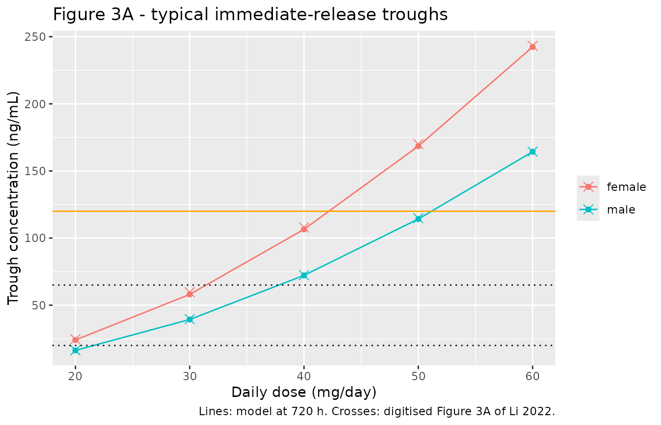
Figure 3A of Li 2022 shows the typical trough concentration of the immediate-release tablet after 20-60 mg once daily in males and females, and Figure 3B the same values divided by the daily dose. The Methods describe the simulation as 100 days of once-daily dosing. The figure is reproduced instead by the trough 24 h after the 30th dose (720 h), as the comparison below shows, so both time points are simulated.
doses <- c(20, 30, 40, 50, 60)
typ_cohort <- tidyr::expand_grid(
  DOSE = doses,
  SEXF = c(0, 1),
  FORM_PAROXETINE_IR = c(1, 0)
) |>
  dplyr::mutate(id = dplyr::row_number())

# 100 days of once-daily dosing into the depot; troughs are read at 720 h
# (24 h after the 30th dose) and 2400 h (24 h after the 100th dose). Dosing
# is into the depot, so Cc is continuous at the dose times and a sample that
# coincides with a dose is still the pre-dose trough.
make_events <- function(cohort, obs_times, n_doses = 100) {
  dose_rows <- cohort |>
    dplyr::mutate(
      time = 0,
      evid = 1L,
      amt = DOSE,
      cmt = "depot",
      ii = 24,
      addl = n_doses - 1L
    )
  obs_rows <- cohort |>
    tidyr::crossing(time = obs_times) |>
    dplyr::mutate(evid = 0L, amt = NA_real_, cmt = "central", ii = 0, addl = 0L)
  # The event columns lead: with a covariate (here DOSE) as the first column
  # of the table, rxSolve() does not pick it up and stops with "required
  # parameter(s): DOSE".
  dplyr::bind_rows(dose_rows, obs_rows) |>
    dplyr::select(id, time, evid, amt, cmt, ii, addl, dplyr::everything()) |>
    dplyr::arrange(id, time, dplyr::desc(evid))
}

ev_typ <- make_events(typ_cohort, obs_times = c(720, 2400))
sim_typ <- rxode2::rxSolve(
  mod_typical,
  events = ev_typ,
  keep = c("DOSE", "SEXF", "FORM_PAROXETINE_IR")
) |>
  as.data.frame()
#> ℹ omega/sigma items treated as zero: 'etalcl', 'etalvc'
#> Warning: multi-subject simulation without without 'omega'
# Figure 3A digitised by the maintainers (immediate-release tablet). Reading
# uncertainty is about 1 ng/mL (one pixel at 300 dpi = 0.46 ng/mL).
fig3a <- tibble::tribble(
  ~DOSE, ~SEXF, ~published,
  20, 0, 16.4,
  30, 0, 39.6,
  40, 0, 72.4,
  50, 0, 114.8,
  60, 0, 164.4,
  20, 1, 24.6,
  30, 1, 59.7,
  40, 1, 107.9,
  50, 1, 169.9,
  60, 1, 243.2
)

fig3_cmp <- sim_typ |>
  dplyr::filter(FORM_PAROXETINE_IR == 1) |>
  dplyr::select(DOSE, SEXF, time, Cc) |>
  tidyr::pivot_wider(names_from = time, values_from = Cc, names_prefix = "t") |>
  dplyr::inner_join(fig3a, by = c("DOSE", "SEXF")) |>
  dplyr::mutate(
    sex = ifelse(SEXF == 1, "female", "male"),
    pct_day30 = 100 * (t720 / published - 1),
    pct_day100 = 100 * (t2400 / published - 1),
    cd_ratio_day30 = t720 / DOSE
  )
stopifnot(nrow(fig3_cmp) == nrow(fig3a))

fig3_cmp |>
  dplyr::select(sex, DOSE, published, t720, pct_day30, t2400, pct_day100, cd_ratio_day30) |>
  dplyr::rename(
    "Sex" = sex,
    "Daily dose (mg)" = DOSE,
    "Figure 3A (ng/mL)" = published,
    "Model, 720 h (ng/mL)" = t720,
    "Diff. 720 h (%)" = pct_day30,
    "Model, 2400 h (ng/mL)" = t2400,
    "Diff. 2400 h (%)" = pct_day100,
    "C/D at 720 h" = cd_ratio_day30
  ) |>
knitr::kable(digits = 2, caption = "Typical immediate-release trough concentrations against Figure 3A of Li 2022.")| Sex | Daily dose (mg) | Figure 3A (ng/mL) | Model, 720 h (ng/mL) | Diff. 720 h (%) | Model, 2400 h (ng/mL) | Diff. 2400 h (%) | C/D at 720 h |
|---|---|---|---|---|---|---|---|
| male | 20 | 16.4 | 16.33 | -0.44 | 16.33 | -0.44 | 0.82 |
| female | 20 | 24.6 | 24.08 | -2.10 | 24.08 | -2.10 | 1.20 |
| male | 30 | 39.6 | 39.34 | -0.65 | 39.38 | -0.55 | 1.31 |
| female | 30 | 59.7 | 58.03 | -2.80 | 58.09 | -2.70 | 1.93 |
| male | 40 | 72.4 | 72.20 | -0.27 | 72.62 | 0.30 | 1.81 |
| female | 40 | 107.9 | 106.50 | -1.30 | 107.11 | -0.73 | 2.66 |
| male | 50 | 114.8 | 114.21 | -0.51 | 116.13 | 1.16 | 2.28 |
| female | 50 | 169.9 | 168.46 | -0.85 | 171.29 | 0.82 | 3.37 |
| male | 60 | 164.4 | 164.31 | -0.05 | 169.98 | 3.39 | 2.74 |
| female | 60 | 243.2 | 242.36 | -0.35 | 250.72 | 3.09 | 4.04 |
The trough at 720 h matches every digitised point within 2.8%. At 2400 h the high-dose points are 3-4% above the figure, because the larger doses have the lowest clearance and are still accumulating at day 30. The 1.475-fold female/male ratio is the sex effect on relative bioavailability, and the C/D column reproduces Figure 3B (male 0.84 to 2.75, female 1.24 to 4.06 as digitised).
# Deterministic typical-value check: no random effects are involved, so the
# only error is the digitisation of Figure 3A (about 1 ng/mL, which is 6% at
# the 16 ng/mL point). A wrong exponent, centring dose, V/F coding or sex
# coding moves these points by 10% or more.
stopifnot(
  max(abs(fig3_cmp$pct_day30)) < 5,
  abs(median(fig3_cmp$pct_day30)) < 2
)
ggplot(fig3_cmp, aes(DOSE, t720, colour = sex)) +
  geom_line() +
  geom_point() +
  geom_point(aes(y = published), shape = 4, size = 3) +
  geom_hline(yintercept = c(20, 65), linetype = "dotted") +
  geom_hline(yintercept = 120, colour = "orange") +
  labs(
    x = "Daily dose (mg/day)",
    y = "Trough concentration (ng/mL)",
    colour = NULL,
    title = "Figure 3A - typical immediate-release troughs",
    caption = "Lines: model at 720 h. Crosses: digitised Figure 3A of Li 2022."
  )
Typical-value replication of Figure 5 (formulation)
Figure 5 of Li 2022 compares the typical immediate-release and sustained-release profiles after 50 mg once daily. The paper’s Methods code the immediate-release tablet as 1, which gives it the smaller V/F (2956 L against 8850 L). The figure confirms that coding: the immediate-release curve swings by about 13 ng/mL across the dosing interval, the sustained-release curve by about 6 ng/mL.
fig5_cohort <- typ_cohort |>
  dplyr::filter(DOSE == 50)
ev_fig5 <- make_events(fig5_cohort, obs_times = seq(696, 744, by = 0.5))
sim_fig5 <- rxode2::rxSolve(
  mod_typical,
  events = ev_fig5,
  keep = c("SEXF", "FORM_PAROXETINE_IR")
) |>
  as.data.frame() |>
  dplyr::mutate(
    sex = ifelse(SEXF == 1, "Female", "Male"),
    formulation = ifelse(FORM_PAROXETINE_IR == 1, "IR-T", "SR-T")
  )
#> ℹ omega/sigma items treated as zero: 'etalcl', 'etalvc'
#> Warning: multi-subject simulation without without 'omega'

ggplot(sim_fig5, aes(time - 696, Cc, linetype = formulation)) +
  geom_line() +
  facet_wrap(~sex) +
  labs(
    x = "Time after the 30th dose (h)",
    y = "Paroxetine (ng/mL)",
    linetype = NULL,
    title = "Figure 5 - 50 mg once daily, days 30-31",
    caption = "Replicates Figure 5 of Li 2022 (typical values)."
  )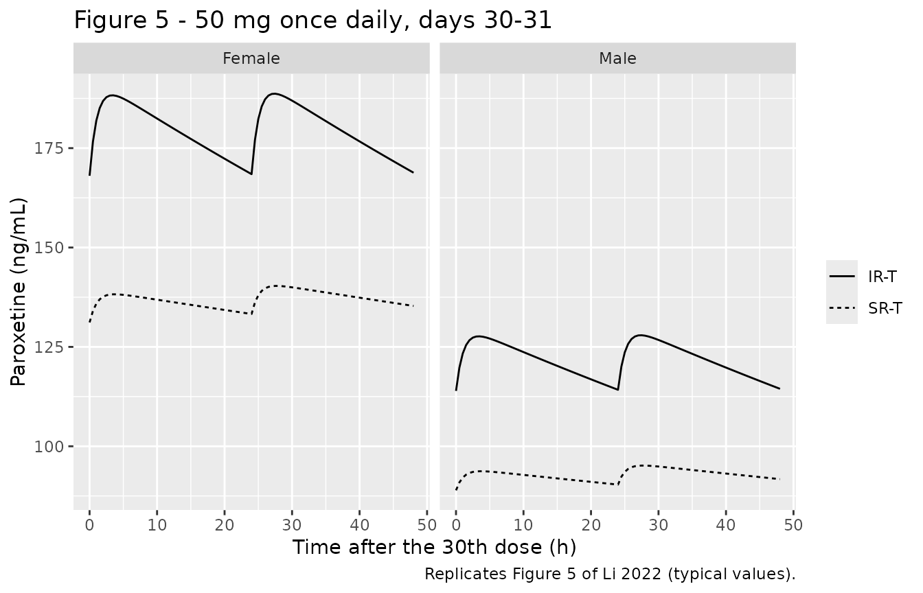
fig5_summary <- sim_fig5 |>
  dplyr::filter(time >= 720, time <= 744) |>
  dplyr::group_by(sex, formulation) |>
  dplyr::summarise(
    trough = Cc[time == 720],
    peak = max(Cc),
    swing = peak - trough,
    .groups = "drop"
  )
knitr::kable(fig5_summary, digits = 1, caption = "Typical trough, peak and peak-trough swing over the 24 h after the 30th dose.")| sex | formulation | trough | peak | swing |
|---|---|---|---|---|
| Female | IR-T | 168.5 | 188.7 | 20.2 |
| Female | SR-T | 133.3 | 140.3 | 7.1 |
| Male | IR-T | 114.2 | 127.9 | 13.7 |
| Male | SR-T | 90.4 | 95.1 | 4.8 |
swing <- function(s, f) fig5_summary$swing[fig5_summary$sex == s & fig5_summary$formulation == f]
trough <- function(s, f) fig5_summary$trough[fig5_summary$sex == s & fig5_summary$formulation == f]
stopifnot(nrow(fig5_summary) == 4L)
# Figure 5 (digitised): male IR-T trough ~115 and swing ~13 ng/mL, SR-T
# trough ~89 and swing ~6 ng/mL. The swing is roughly F * dose / (V/F), so it
# is the direct test of which formulation carries the 0.334 factor on V/F.
stopifnot(
  abs(trough("Male", "IR-T") / 115 - 1) < 0.05,
  abs(trough("Male", "SR-T") / 89 - 1) < 0.05,
  swing("Male", "IR-T") / swing("Male", "SR-T") > 2
)
At true steady state the two tablets have the same average concentration, because formulation enters only V/F. The lower sustained-release trough in Figures 4 and 5 of the paper comes from the larger V/F: at 50 mg the sustained-release half-life is 15 days, so at day 30 it is still accumulating. By day 100 the typical sustained-release trough (120 ng/mL for a male) is slightly above the immediate-release one (116 ng/mL).
Stochastic replication of Figure 4
Figure 4 of Li 2022 shows box plots of simulated troughs (individual predictions, no residual error) for 25 and 50 mg once daily by sex and formulation. A virtual cohort of 100 patients per arm (8 arms) is simulated with between-subject variability and the trough read at 720 h, matching the time point that reproduces Figures 3 and 5.
rxode2::rxSetSeed(20220912)
n_per_arm <- 100L
fig4_cohort <- tidyr::expand_grid(
  DOSE = c(25, 50),
  SEXF = c(0, 1),
  FORM_PAROXETINE_IR = c(1, 0),
  rep = seq_len(n_per_arm)
) |>
  dplyr::mutate(id = dplyr::row_number()) |>
  dplyr::select(-rep)
ev_fig4 <- make_events(fig4_cohort, obs_times = 720)
stopifnot(!anyDuplicated(unique(ev_fig4[, c("id", "time", "evid")])))

sim_fig4 <- rxode2::rxSolve(
  mod,
  events = ev_fig4,
  keep = c("DOSE", "SEXF", "FORM_PAROXETINE_IR")
) |>
  as.data.frame() |>
  dplyr::mutate(
    sex = ifelse(SEXF == 1, "female", "male"),
    formulation = ifelse(FORM_PAROXETINE_IR == 1, "immediate-release tablet", "sustained-release tablet"),
    dose = paste(DOSE, "mg")
  )
#> ℹ parameter labels from comments will be replaced by 'label()'
stopifnot(!anyNA(sim_fig4$Cc))

ggplot(sim_fig4, aes(sex, Cc, fill = formulation)) +
  geom_boxplot(outlier.size = 0.5) +
  facet_wrap(~dose) +
  geom_hline(yintercept = c(20, 65), linetype = "dashed") +
  geom_hline(yintercept = 120, colour = "red", linetype = "dashed") +
  labs(
    x = NULL,
    y = "Simulated trough (ng/mL)",
    fill = NULL,
    title = "Figure 4 - simulated troughs at 720 h",
    caption = "Replicates Figure 4 of Li 2022 (100 virtual patients per arm, individual predictions)."
  ) +
  theme(legend.position = "bottom")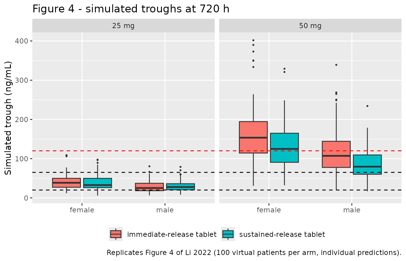
# Figure 4 box-plot medians digitised by the maintainers.
fig4_pub <- tibble::tribble(
  ~DOSE, ~SEXF, ~FORM_PAROXETINE_IR, ~published_median,
  25, 0, 1, 23.8,
  25, 0, 0, 21.0,
  25, 1, 1, 36.5,
  25, 1, 0, 33.0,
  50, 0, 1, 98.9,
  50, 0, 0, 75.0,
  50, 1, 1, 147.3,
  50, 1, 0, 110.8
)
fig4_cmp <- sim_fig4 |>
  dplyr::group_by(DOSE, SEXF, FORM_PAROXETINE_IR, sex, formulation) |>
  dplyr::summarise(sim_median = median(Cc), .groups = "drop") |>
  dplyr::inner_join(fig4_pub, by = c("DOSE", "SEXF", "FORM_PAROXETINE_IR")) |>
  dplyr::mutate(pct_diff = 100 * (sim_median / published_median - 1))
stopifnot(nrow(fig4_cmp) == 8L)

fig4_cmp |>
  dplyr::select(DOSE, sex, formulation, published_median, sim_median, pct_diff) |>
  dplyr::rename(
    "Daily dose (mg)" = DOSE,
    "Sex" = sex,
    "Formulation" = formulation,
    "Figure 4 median (ng/mL)" = published_median,
    "Simulated median (ng/mL)" = sim_median,
    "Difference (%)" = pct_diff
  ) |>
knitr::kable(digits = 1, caption = "Median simulated trough at 720 h against Figure 4 of Li 2022.")| Daily dose (mg) | Sex | Formulation | Figure 4 median (ng/mL) | Simulated median (ng/mL) | Difference (%) |
|---|---|---|---|---|---|
| 25 | male | sustained-release tablet | 21.0 | 27.6 | 31.6 |
| 25 | male | immediate-release tablet | 23.8 | 25.2 | 5.7 |
| 25 | female | sustained-release tablet | 33.0 | 32.6 | -1.1 |
| 25 | female | immediate-release tablet | 36.5 | 38.5 | 5.4 |
| 50 | male | sustained-release tablet | 75.0 | 79.6 | 6.1 |
| 50 | male | immediate-release tablet | 98.9 | 107.2 | 8.3 |
| 50 | female | sustained-release tablet | 110.8 | 124.8 | 12.7 |
| 50 | female | immediate-release tablet | 147.3 | 153.5 | 4.2 |
ratio_ir_sr <- sim_fig4 |>
  dplyr::filter(DOSE == 50) |>
  dplyr::group_by(FORM_PAROXETINE_IR) |>
  dplyr::summarise(m = median(Cc / (1 + 0.475 * SEXF)), .groups = "drop")
ratio_ir_sr <- ratio_ir_sr$m[ratio_ir_sr$FORM_PAROXETINE_IR == 1] /
  ratio_ir_sr$m[ratio_ir_sr$FORM_PAROXETINE_IR == 0]
Across the eight arms the simulated medians differ from the digitised Figure 4 medians by -1% to 32% (median 6%). Each arm median from 100 virtual patients has a sampling error of about 6%, the 25 mg arms sit at 20-40 ng/mL where reading the figure is least precise, and the paper built its cohorts by resampling individual predictions of its own patients rather than drawing fresh random effects, so single-arm differences of this size are expected. The immediate-release to sustained-release ratio of the medians at 50 mg (1.28, sex-normalised) matches the figure (98.9/75.0 = 1.32 in males, 147.3/110.8 = 1.33 in females).
# Centre and ratio only (CLAUDE.md: never gate the extremes of a cohort).
# With 100 per arm the SE of a log-median is about 1.25 * 0.5 / 10 = 6%, so
# the IR/SR ratio of the 200-patient pooled medians has an SE near 0.06; the
# 1.05-1.60 window is more than 3 SE either side of the 1.26 typical-value
# ratio at day 30. A swapped formulation coding gives about 0.8, which fails.
# The median of the eight per-arm differences (about 6% on the authoring run,
# each arm with a ~6% sampling SE) is gated at 15%: a mis-transcribed CL/F,
# dose exponent or F moves every arm by 20% or more.
stopifnot(
  ratio_ir_sr > 1.05,
  ratio_ir_sr < 1.60,
  abs(median(fig4_cmp$pct_diff)) < 15
)
PKNCA validation at steady state
Li 2022 reports no non-compartmental results, so the NCA check is
internal: PKNCA is run on the typical-value profiles over the 100th
dosing interval (2376-2400 h) and the average concentration is compared
against the closed-form steady-state value
F * dose / (CL/F * tau), which depends only on the dose
exponent, the sex effect on F and the clearance.
ev_ss <- make_events(typ_cohort, obs_times = c(0, seq(2376, 2400, by = 0.25)))
sim_ss <- rxode2::rxSolve(
  mod_typical,
  events = ev_ss,
  keep = c("DOSE", "SEXF", "FORM_PAROXETINE_IR")
) |>
  as.data.frame() |>
  dplyr::mutate(
    treatment = paste0(
      ifelse(FORM_PAROXETINE_IR == 1, "IR-T ", "SR-T "), DOSE, " mg, ",
      ifelse(SEXF == 1, "female", "male")
    )
  )
#> ℹ omega/sigma items treated as zero: 'etalcl', 'etalvc'
#> Warning: multi-subject simulation without without 'omega'

conc_df <- sim_ss |>
  dplyr::filter(!is.na(Cc)) |>
  dplyr::mutate(Cc = pmax(Cc, 0)) |>
  dplyr::select(id, time, Cc, treatment)

dose_df <- ev_ss |>
  dplyr::filter(evid == 1) |>
  dplyr::select(id, DOSE, SEXF, FORM_PAROXETINE_IR, amt, ii, addl) |>
  tidyr::uncount(addl + 1L, .id = "n") |>
  dplyr::mutate(
    time = (n - 1) * ii,
    treatment = paste0(
      ifelse(FORM_PAROXETINE_IR == 1, "IR-T ", "SR-T "), DOSE, " mg, ",
      ifelse(SEXF == 1, "female", "male")
    )
  ) |>
  dplyr::select(id, time, amt, treatment)

conc_obj <- PKNCA::PKNCAconc(conc_df, Cc ~ time | treatment + id)
dose_obj <- PKNCA::PKNCAdose(dose_df, amt ~ time | treatment + id)
intervals <- data.frame(
  start = 2376,
  end = 2400,
  cmax = TRUE,
  tmax = TRUE,
  cmin = TRUE,
  cav = TRUE
)
nca_res <- PKNCA::pk.nca(PKNCA::PKNCAdata(conc_obj, dose_obj, intervals = intervals))

nca_wide <- as.data.frame(nca_res$result) |>
  dplyr::select(treatment, PPTESTCD, PPORRES) |>
  tidyr::pivot_wider(names_from = PPTESTCD, values_from = PPORRES) |>
  dplyr::left_join(
    sim_ss |> dplyr::distinct(treatment, DOSE, SEXF, FORM_PAROXETINE_IR),
    by = "treatment"
  ) |>
  dplyr::mutate(
    cav_closed = 1000 * (1 + 0.475 * SEXF) * DOSE / (21.2 * (DOSE / 40)^-1.03 * 24),
    pct_diff = 100 * (cav / cav_closed - 1)
  ) |>
  dplyr::arrange(FORM_PAROXETINE_IR, SEXF, DOSE)

nca_wide |>
  dplyr::select(treatment, cmax, tmax, cmin, cav, cav_closed, pct_diff) |>
  dplyr::rename(
    "Group" = treatment,
    "Cmax,ss (ng/mL)" = cmax,
    "Tmax (h after dose)" = tmax,
    "Cmin,ss (ng/mL)" = cmin,
    "Cav,ss PKNCA (ng/mL)" = cav,
    "Cav,ss closed form (ng/mL)" = cav_closed,
    "Difference (%)" = pct_diff
  ) |>
knitr::kable(digits = 2, caption = "Steady-state NCA over the 100th dosing interval (typical values).")| Group | Cmax,ss (ng/mL) | Tmax (h after dose) | Cmin,ss (ng/mL) | Cav,ss PKNCA (ng/mL) | Cav,ss closed form (ng/mL) | Difference (%) |
|---|---|---|---|---|---|---|
| SR-T 20 mg, male | 20.07 | 3.25 | 18.24 | 19.25 | 19.25 | 0.00 |
| SR-T 30 mg, male | 45.05 | 3.25 | 42.30 | 43.82 | 43.84 | -0.05 |
| SR-T 40 mg, male | 79.99 | 3.50 | 76.32 | 78.36 | 78.62 | -0.32 |
| SR-T 50 mg, male | 124.39 | 3.50 | 119.80 | 122.38 | 123.66 | -1.04 |
| SR-T 60 mg, male | 177.37 | 3.50 | 171.84 | 174.98 | 179.05 | -2.27 |
| SR-T 20 mg, female | 29.60 | 3.25 | 26.90 | 28.39 | 28.39 | 0.00 |
| SR-T 30 mg, female | 66.44 | 3.25 | 62.39 | 64.64 | 64.67 | -0.05 |
| SR-T 40 mg, female | 117.98 | 3.50 | 112.57 | 115.59 | 115.96 | -0.32 |
| SR-T 50 mg, female | 183.48 | 3.50 | 176.70 | 180.51 | 182.40 | -1.04 |
| SR-T 60 mg, female | 261.62 | 3.50 | 253.47 | 258.10 | 264.10 | -2.27 |
| IR-T 20 mg, male | 21.77 | 3.25 | 16.33 | 19.25 | 19.25 | -0.01 |
| IR-T 30 mg, male | 47.57 | 3.25 | 39.38 | 43.84 | 43.84 | 0.00 |
| IR-T 40 mg, male | 83.56 | 3.25 | 72.62 | 78.61 | 78.62 | 0.00 |
| IR-T 50 mg, male | 129.82 | 3.25 | 116.13 | 123.66 | 123.66 | 0.00 |
| IR-T 60 mg, male | 186.41 | 3.25 | 169.98 | 179.05 | 179.05 | 0.00 |
| IR-T 20 mg, female | 32.11 | 3.25 | 24.08 | 28.39 | 28.39 | -0.01 |
| IR-T 30 mg, female | 70.17 | 3.25 | 58.09 | 64.66 | 64.67 | 0.00 |
| IR-T 40 mg, female | 123.25 | 3.25 | 107.11 | 115.96 | 115.96 | 0.00 |
| IR-T 50 mg, female | 191.48 | 3.25 | 171.29 | 182.40 | 182.40 | 0.00 |
| IR-T 60 mg, female | 274.96 | 3.25 | 250.71 | 264.09 | 264.10 | 0.00 |
# The 0.25 h linear-up/log-down trapezoid on a profile this flat is accurate
# to well under 0.5%; residual accumulation at day 100 (largest for SR-T at
# 60 mg, half-life about 18 days, exp(-99 / 25.9) < 2.5%) is the only other
# contribution and it can only lower the PKNCA value.
stopifnot(
  nrow(nca_wide) == nrow(typ_cohort),
  all(nca_wide$pct_diff < 0.5),
  all(nca_wide$pct_diff > -4)
)
The steady-state peak-to-trough ratio is small for both tablets (half-lives of days), which is why trough concentrations taken 10-22.5 h after the dose are a good summary of exposure in this TDM population.
Assumptions and deviations
-
Formulation coding. The Methods code the
immediate-release tablet as 1 and the printed equation applies
(1 - 0.666 * formulation)to V/F, giving the immediate-release tablet the smaller V/F (2956 L). The Abstract and Discussion describe the effect the other way round (“the SR-T resulted in a decrease in V/F of about 66.6%”). The Methods coding was kept because it is the one under which the paper’s own typical-value simulations (Figure 3A and the peak-trough swings in Figure 5) are reproduced; under the Discussion’s orientation the 720 h immediate-release troughs would differ from Figure 3A by +8% at 20 mg to -27% at 60 mg, and the Figure 5 swings would be exchanged. - Simulation horizon of the published figures. The Methods state 100 days of once-daily dosing, but Figures 3A and 5 are reproduced by the trough 24 h after the 30th dose. The library model is unaffected; this vignette compares at 720 h and also reports 2400 h.
- Figure 4 cohorts. The paper built Figure 4 by resampling individual predictions from its own patients, which cannot be reproduced without the data; this vignette draws fresh random effects from the reported IIV instead. Only the centre of the per-arm differences and the formulation ratio are gated, not single arms.
-
IIV scale. Table 2 gives IIV as CV% without stating
the conversion. The variances use
omega^2 = log(1 + CV^2). The alternative readingomega^2 = (CV/100)^2would give 0.269 (CL/F) and 0.697 (V/F); the paper reports no confidence intervals on the IIV rows that could separate the two readings. -
Residual error scale. Table 2 prints the
proportional residual error as ‘PRO (CV%) 0.0929’ while the IIV rows in
the same table are printed as percentages. The value was read as the raw
NONMEM
$SIGMAvariance, giving a proportional SD of 0.305 (30.5%). If it were already an SD the residual error would be 9.3%; the residual error does not enter any of the typical-value or individual-prediction checks above. -
Daily dose covariate.
DOSEis the total daily dose in mg. The paper centres it at 40 mg/day; the reported dose range is 20-75 mg/day, and the power model should not be extrapolated far outside it (at 10 mg/day the predicted CL/F would be 89 L/h). - Typographical error in the Results. The Results state that males require “at least 5 mg QD” to reach a 20 ng/mL trough; with the model the typical male needs between 20 and 25 mg/day, consistent with the Discussion’s statement that 20 mg/day in females corresponds to 25 mg/day in males.
- No erratum or correction notice for Li 2022 was indexed in Europe PMC as of 2026-10-09.