Brigatinib (Hanley 2024)
Source:vignettes/articles/Hanley_2024_brigatinib.Rmd
Hanley_2024_brigatinib.RmdModel and source
- Citation: Hanley MJ, Rowland Yeo K, Tugnait M, Iwasaki S, Narasimhan N, Zhang P, Venkatakrishnan K, Gupta N. (2024). Evaluation of the drug-drug interaction potential of brigatinib using a physiologically-based pharmacokinetic modeling approach. CPT Pharmacometrics Syst Pharmacol 13(4):624-637. doi:10.1002/psp4.13106.
- Description: Two-compartment oral population pharmacokinetic reduction of the Simcyp minimal-PBPK-with-single-adjusting-compartment (SAC) model for the ALK inhibitor brigatinib in healthy adults (Hanley 2024). The source model was built in the Simcyp Population-based Simulator (versions 15 and 17) and its whole-body mass-balance equations are not published, so the platform model itself cannot be encoded here. What IS fully reported is the brigatinib compound layer, and it is sufficient to reconstruct the disposition as an ordinary compartmental model: first-order absorption into a depot, distribution between a systemic compartment and the SAC (the paper’s k_in / k_out, encoded as the canonical k12 / k21), and first-order elimination from the systemic compartment. Systemic clearance is obtained from the reported unbound hepatic intrinsic clearance through the well-stirred liver model plus the reported renal clearance; bioavailability is the reported f_a times f_G times the f_H implied by that same well-stirred calculation. No parameter is fitted here and none is imported from a Simcyp population file: every value is either a Table 1 / Appendix S1 input or an arithmetic consequence of one. The reduction reproduces the paper’s own predicted Cmax, Tmax and AUC after single 90 mg and 180 mg oral doses to within 6.4%, and Cmax at both doses to within 1% (see the validation vignette). This is a typical-value simulation model: the source reports no inter-individual variance components and no residual-error model, so there are no etas and propSd is fixed at zero. The drug-drug-interaction predictions that are the paper’s main contribution (itraconazole, rifampin, diltiazem, verapamil, efavirenz, and the transporter substrates) depend on proprietary Simcyp perpetrator compound files and are NOT reproducible from this model; see the vignette for the full list of deviations.
- Article: https://doi.org/10.1002/psp4.13106
- Supplement (Appendix S1): https://www.ncbi.nlm.nih.gov/pmc/articles/PMC11015081/
What this model is, and what it is not
Hanley 2024 built a minimal PBPK model with a single adjusting compartment (SAC) for brigatinib in the Simcyp Population-based Simulator (versions 15 and 17), and used it to predict drug-drug interactions (DDIs) with CYP3A inhibitors and inducers and with transporter substrates.
Simcyp’s whole-body mass-balance equations are proprietary and are not printed in the paper or in Appendix S1 – Figure 1b is a box-and-arrow schematic, and the seven numbered equations in the supplement are all input-derivation formulae (partition-coefficient prediction, retrograde clearance, ISEF scaling, Cheng-Prusoff, population-file calibration), never the disposition ODEs. The platform model therefore cannot be encoded as published.
What is completely reported is the brigatinib compound layer: the absorption parameters, the distribution parameters that define the SAC, the unbound hepatic intrinsic clearance, the renal clearance, and the physiological scalars needed to turn those into a systemic clearance. Those are enough to rebuild the disposition as an ordinary two-compartment oral model. That reduction is what this package ships, and the sections below show that it reproduces the paper’s own predicted Cmax, Tmax, and AUC to within 6.4%, without a single fitted parameter.
The DDI predictions are not reproducible. Every result in Tables 2 (test arms), 3, and 4 depends on Simcyp compound files for itraconazole, hydroxy-itraconazole, rifampin, diltiazem, verapamil, efavirenz, digoxin, dabigatran, rosuvastatin, and metformin that are proprietary to Certara. This model reproduces the brigatinib control arms only. See Assumptions and deviations.
Population
The model inputs were assembled from six clinical studies of brigatinib (Hanley 2024 Methods, “Clinical data for brigatinib”; Appendix S1):
-
AP26113-15-106 – an open-label, randomized,
two-period bioequivalence crossover study in 36 healthy participants.
This is the study the disposition parameters (
ka, Vss, Vsac,kin,kout) were optimized against, and the study whose observed oral clearance of 13.47 L/h anchors the retrograde clearance calculation. - AP26113-13-104 – a human ADME / mass balance study in six healthy male participants given a single 180 mg / 100 uCi [14C]-brigatinib dose. The recovery split (89.75% total; 24.99% urine, 64.76% faeces; 40.91% of faecal radioactivity as unchanged brigatinib) fixes the fraction absorbed at 0.63 and the renal fraction at 21.38% of the dose.
- AP26113-15-105 – a three-arm, open-label, randomized, fixed-sequence crossover DDI study (n = 20 per arm) with gemfibrozil, itraconazole, and rifampin.
- AP26113-15-107 (hepatic impairment) and AP26113-15-108 (renal impairment) – contributed ex vivo plasma protein binding from 17 pooled healthy participants, giving a mean bound fraction of 91.17% and hence fu = 0.0883.
- AP26113-11-101 (NCT01449461) – the phase I/II study in patients with ALK-positive advanced malignancies used for the multiple-dose verification arm.
Simulations of healthy participants used the Simcyp default North European Caucasian population; the cancer arm used the Simcyp Sim-Cancer population described in Appendix S1.
The same information is available programmatically via
readModelDb("Hanley_2024_brigatinib")()$population.
Source trace
Every value in ini() is either a verbatim Hanley 2024
Table 1 / Appendix S1 input or an arithmetic consequence of one. Nothing
was fitted.
| Parameter / equation | Value | Source location |
|---|---|---|
lka |
1.8 1/h | Table 1 (ka); Appendix S1 “Determination of absorption
parameters” – sensitivity analysis to recover the observed ~2 h
Tmax |
lk12 |
28.13 1/h | Table 1 (kin, “first-order rate constant that acts on
the masses of drug within the systemic compartment”); Figure 1
legend |
lk21 |
20.00 1/h | Table 1 (kout, “acts on the masses of drug within the
SAC”); Figure 1 legend |
lvc |
62.05 L | Derived: (Vss 6.91 - Vsac 6.0) L/kg x 70 kg - 1.648 L liver. Table 1 for the two volumes; Appendix S1 Eq. S2 for the 1648 g default liver weight |
lcl |
7.1816 L/h | Derived: well-stirred hepatic clearance from Table 1 (CLuH,int 12.21 uL/min/mg, fu 0.0883, B:P 0.69) plus Table 1 renal clearance 3.21 L/h. Appendix S1 Eq. S2 supplies QH = 90 L/h, liver 1648 g, 39.8 mg protein/g liver |
lfdepot |
0.5307 | Derived: fa 0.63 (Table 1) x fG 0.9 (Appendix S1 Eq. S2 text) x fH 0.936 (from the same well-stirred calculation) |
propSd |
0 (fixed) | Not reported. Hanley 2024 is a PBPK simulation analysis with no residual-error model and no estimated variance components |
d/dt(depot), d/dt(central),
d/dt(peripheral1)
|
n/a | Figure 1b schematic plus the Figure 1 legend definitions of
kin and kout, with the liver and portal-vein
compartments lumped into the systemic compartment |
Reproducing the two derivations
The clearance and volume derivations are the only places where this model departs from transcription, so they are recomputed here from the published inputs and checked against the packaged values.
# --- Published inputs (Hanley 2024 Table 1 and Appendix S1) ---------------
fu             <- 0.0883   # Table 1, fraction unbound in plasma
bp             <- 0.69     # Table 1, blood-to-plasma ratio
clint_per_mg   <- 12.21    # Table 1, CLuH,int (uL/min/mg microsomal protein)
clr            <- 3.21     # Table 1, renal clearance (L/h)
qh             <- 90       # Appendix S1 Eq. S2, hepatic blood flow (L/h)
liver_g        <- 1648     # Appendix S1 Eq. S2, default liver weight (g)
mppgl          <- 39.8     # Appendix S1 Eq. S2, mg microsomal protein / g liver
fa             <- 0.63     # Table 1, fraction absorbed
fg             <- 0.9      # Appendix S1 Eq. S2 text, fraction escaping the gut
vss_per_kg     <- 6.91     # Table 1, whole-body steady-state volume (L/kg)
vsac_per_kg    <- 6.0      # Table 1, SAC volume (L/kg)
bw_ref         <- 70       # reference body weight (kg) for the L/kg inputs
clf_observed   <- 13.47    # Appendix S1 Eq. S2 text, observed CL/F (L/h)

# --- Whole-liver unbound intrinsic clearance ------------------------------
# uL/min/mg * mg/g * g -> uL/min; /1e6 -> L/min; *60 -> L/h
clint_lh <- clint_per_mg * mppgl * liver_g / 1e6 * 60
fub      <- fu / bp

# --- Well-stirred liver ---------------------------------------------------
cl_h_blood  <- qh * fub * clint_lh / (qh + fub * clint_lh)
fh          <- qh / (qh + fub * clint_lh)
cl_h_plasma <- cl_h_blood * bp
cl_total    <- cl_h_plasma + clr
fbio        <- fa * fg * fh

# --- Systemic compartment volume -----------------------------------------
vc <- (vss_per_kg - vsac_per_kg) * bw_ref - liver_g / 1000

tibble::tibble(
  Quantity = c("CLuH,int (whole liver, L/h)", "fu,blood", "fH",
               "Hepatic CL (plasma, L/h)", "Total CL (L/h)",
               "F = fa * fG * fH", "vc (L)"),
  Value = round(c(clint_lh, fub, fh, cl_h_plasma, cl_total, fbio, vc), 4)
) |>
knitr::kable(caption = "Derived parameters recomputed from the published inputs.")| Quantity | Value |
|---|---|
| CLuH,int (whole liver, L/h) | 48.0515 |
| fu,blood | 0.1280 |
| fH | 0.9360 |
| Hepatic CL (plasma, L/h) | 3.9716 |
| Total CL (L/h) | 7.1816 |
| F = fa * fG * fH | 0.5307 |
| vc (L) | 62.0520 |
These must agree with what the packaged model carries:
ini_vals <- rxode2::rxode(readModelDb("Hanley_2024_brigatinib"))$iniDf
packaged <- setNames(exp(ini_vals$est), ini_vals$name)

stopifnot(
  abs(packaged[["lcl"]]     - cl_total) < 0.01,
  abs(packaged[["lvc"]]     - vc)       < 0.01,
  abs(packaged[["lfdepot"]] - fbio)     < 0.001,
  abs(packaged[["lka"]]     - 1.8)      < 1e-8,
  abs(packaged[["lk12"]]    - 28.13)    < 1e-8,
  abs(packaged[["lk21"]]    - 20.00)    < 1e-8
)
cat("Packaged ini() values match the derivation from the published inputs.\n")
#> Packaged ini() values match the derivation from the published inputs.
Erratum: the 43.02 L/h in Appendix S1 is a transcription error
Appendix S1 states that the retrograde calculation gave a total CLuH,int of “43.02 L/h”, which it then rescales to the 12.21 uL/min/mg value that appears in Table 1. Those two numbers are not consistent with each other, and it is 43.02 that is wrong: the rescaling scalars printed in the same sentence turn 12.21 uL/min/mg into 48.05 L/h, and only 48.05 L/h reproduces the observed oral clearance the retrograde equation was solved against.
retrograde_clf <- function(clint_lh) {
  x  <- (fu / bp) * clint_lh
  fh <- qh / (qh + x)
  (qh * x / (qh + x) * bp + clr) / (fa * fg * fh)
}

tibble::tibble(
  `CLuH,int (L/h)` = c(48.05, 43.02),
  Source = c("implied by Table 1's 12.21 uL/min/mg",
             "as printed in Appendix S1"),
  `CL/F returned (L/h)` = round(retrograde_clf(c(48.05, 43.02)), 2),
  `vs observed 13.47` = paste0(
    round(100 * (retrograde_clf(c(48.05, 43.02)) / clf_observed - 1), 1), "%")
) |>
knitr::kable(caption = "Only 48.05 L/h recovers the observed CL/F of 13.47 L/h.")| CLuH,int (L/h) | Source | CL/F returned (L/h) | vs observed 13.47 |
|---|---|---|---|
| 48.05 | implied by Table 1’s 12.21 uL/min/mg | 13.53 | 0.5% |
| 43.02 | as printed in Appendix S1 | 12.71 | -5.7% |
The value actually entered into Simcyp is the Table 1 figure of 12.21 uL/min/mg – it is also the figure apportioned across metabolic pathways in Appendix S1 Table S3, whose entries sum to 12.21 – so the model is unaffected by the typo. This model uses 48.05 L/h.
Virtual cohort
The model has no random effects and no covariates, so it is deterministic: one subject per arm fully characterises each scenario, and there is nothing for a larger cohort to add. Observed individual concentrations from the source figures were not digitised, so the comparisons below are against the paper’s predicted summary statistics in Table 2.
Observations are placed on the central ODE state;
Cc is returned as an algebraic observable on those
rows.
obs_grid <- sort(unique(c(
  seq(0, 6, by = 0.05),      # dense through Tmax
  seq(6, 24, by = 0.25),
  seq(24, 120, by = 1)
)))

make_single_dose <- function(id, dose, label) {
  dplyr::bind_rows(
    tibble::tibble(id = id, time = 0, amt = dose, evid = 1L,
                   cmt = "depot", arm = label),
    tibble::tibble(id = id, time = obs_grid, amt = NA_real_, evid = 0L,
                   cmt = "central", arm = label)
  )
}

events_sd <- dplyr::bind_rows(
  make_single_dose(1L,  90, "90 mg single dose"),
  make_single_dose(2L, 180, "180 mg single dose")
) |>
  dplyr::arrange(id, time, dplyr::desc(evid))

stopifnot(!anyDuplicated(events_sd[, c("id", "time", "evid")]))
Simulation
mod <- readModelDb("Hanley_2024_brigatinib")
sim_sd <- rxode2::rxSolve(mod, events = events_sd, keep = "arm")
#> Warning: multi-subject simulation without without 'omega'
Replicate published figures
# Replicates the model-predicted mean line of Figure 2a of Hanley 2024
# (single oral 90 mg dose in healthy participants). The observed individual
# concentrations and the 5th/95th percentile band of Figure 2a are driven by
# the Simcyp virtual population and are not reproducible here.
sim_sd |>
  dplyr::filter(arm == "90 mg single dose", Cc > 0) |>
  ggplot(aes(time, Cc)) +
  geom_line(linewidth = 0.8) +
  scale_y_log10() +
  scale_x_continuous(breaks = seq(0, 120, by = 24)) +
  labs(x = "Time (h)", y = "Brigatinib concentration (ng/mL)",
       title = "Predicted plasma brigatinib after a single 90 mg oral dose",
       caption = "Compare with the mean prediction line of Figure 2a of Hanley 2024.")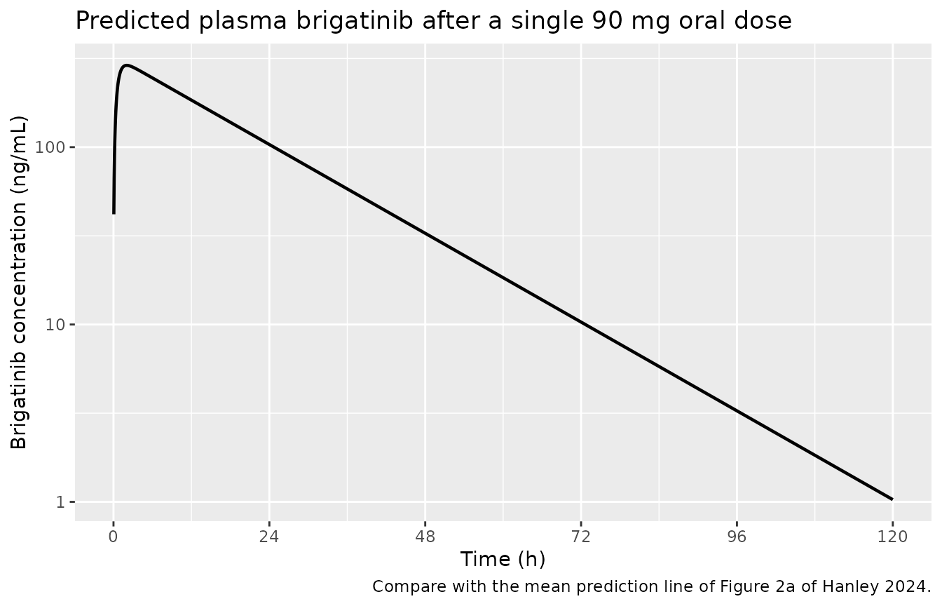
sim_sd |>
  dplyr::filter(Cc > 0) |>
  ggplot(aes(time, Cc, colour = arm)) +
  geom_line(linewidth = 0.8) +
  scale_y_log10() +
  scale_x_continuous(limits = c(0, 48), breaks = seq(0, 48, by = 12)) +
  labs(x = "Time (h)", y = "Brigatinib concentration (ng/mL)",
       colour = NULL,
       title = "Dose proportionality over the two studied single doses")
#> Warning: Removed 144 rows containing missing values or values outside the scale range
#> (`geom_line()`).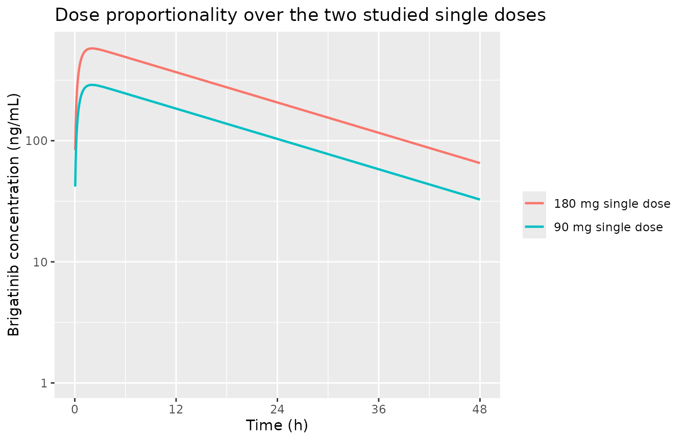
Brigatinib PK was dose-linear over 60-240 mg (Hanley 2024 Discussion), and the reduction is a linear model, so the 180 mg profile must be exactly twice the 90 mg profile:
wide <- sim_sd |>
  dplyr::select(arm, time, Cc) |>
  tidyr::pivot_wider(names_from = arm, values_from = Cc)
ratio <- wide[["180 mg single dose"]] / wide[["90 mg single dose"]]
ratio <- ratio[is.finite(ratio)]
# Tolerance is relative and set by the ODE solver, not by the model: the
# ratio is 2 analytically, and the residual ~2e-6 is integration error.
stopifnot(all(abs(ratio / 2 - 1) < 1e-4))
cat(sprintf(paste("Dose linearity holds: 180 mg / 90 mg concentration ratio",
                  "= 2 to within %.1e (relative).\n"),
            max(abs(ratio / 2 - 1))))
#> Dose linearity holds: 180 mg / 90 mg concentration ratio = 2 to within 1.7e-06 (relative).
PKNCA validation
conc_sd <- sim_sd |>
  dplyr::filter(!is.na(Cc)) |>
  dplyr::select(id, time, Cc, arm)

# Guarantee a time-zero record per subject (pre-dose Cc = 0 for oral dosing).
conc_sd <- dplyr::bind_rows(
  conc_sd,
  conc_sd |> dplyr::distinct(id, arm) |> dplyr::mutate(time = 0, Cc = 0)
) |>
  dplyr::distinct(id, arm, time, .keep_all = TRUE) |>
  dplyr::arrange(id, arm, time)

dose_sd <- events_sd |>
  dplyr::filter(evid == 1L) |>
  dplyr::select(id, time, amt, arm)

conc_obj <- PKNCA::PKNCAconc(conc_sd, Cc ~ time | arm + id,
                             concu = "ng/mL", timeu = "h")
dose_obj <- PKNCA::PKNCAdose(dose_sd, amt ~ time | arm + id, doseu = "mg")

intervals_sd <- data.frame(
  start      = c(0, 0),
  end        = c(120, Inf),
  cmax       = c(TRUE,  FALSE),
  tmax       = c(TRUE,  FALSE),
  auclast    = c(TRUE,  FALSE),
  aucinf.obs = c(FALSE, TRUE),
  half.life  = c(FALSE, TRUE)
)

nca_sd <- PKNCA::pk.nca(
  PKNCA::PKNCAdata(conc_obj, dose_obj, intervals = intervals_sd)
)

knitr::kable(
  as.data.frame(nca_sd) |>
    dplyr::filter(PPTESTCD %in% c("cmax", "tmax", "auclast",
                                  "aucinf.obs", "half.life")) |>
    dplyr::mutate(PPORRES = signif(PPORRES, 4)) |>
    dplyr::select(arm, start, end, PPTESTCD, PPORRES),
  caption = "PKNCA results for the simulated single-dose arms."
)| arm | start | end | PPTESTCD | PPORRES |
|---|---|---|---|---|
| 180 mg single dose | 0 | 120 | auclast | 13260.00 |
| 180 mg single dose | 0 | 120 | cmax | 578.50 |
| 180 mg single dose | 0 | 120 | tmax | 2.05 |
| 180 mg single dose | 0 | Inf | tmax | 2.05 |
| 180 mg single dose | 0 | Inf | half.life | 14.44 |
| 180 mg single dose | 0 | Inf | aucinf.obs | 13300.00 |
| 90 mg single dose | 0 | 120 | auclast | 6629.00 |
| 90 mg single dose | 0 | 120 | cmax | 289.20 |
| 90 mg single dose | 0 | 120 | tmax | 2.05 |
| 90 mg single dose | 0 | Inf | tmax | 2.05 |
| 90 mg single dose | 0 | Inf | half.life | 14.44 |
| 90 mg single dose | 0 | Inf | aucinf.obs | 6650.00 |
Comparison against the published NCA
Hanley 2024 Table 2 reports model-predicted values for both single doses. The 90 mg Cmax, Tmax, and AUC120 come from the bioequivalence-study row (AP26113-15-106); the 90 mg AUC-infinity is taken from the itraconazole control arm, which is the only 90 mg AUC-infinity the paper reports, and which was simulated in a slightly different virtual population (predicted Cmax 279 ng/mL there, versus 292 ng/mL in the bioequivalence-study row). The 180 mg values are the rifampin control arm. Tmax and AUC120 were not reported for 180 mg.
published_sd <- tibble::tribble(
  ~arm,                  ~cmax, ~tmax, ~auclast, ~aucinf.obs,
  "90 mg single dose",     292,   2.1,     6825,        6927,
  "180 mg single dose",    581,    NA,       NA,       14205
)

cmp_sd <- nlmixr2lib::ncaComparisonTable(
  simulated = as.data.frame(nca_sd) |>
    dplyr::filter(PPTESTCD %in% c("cmax", "tmax", "auclast", "aucinf.obs")),
  reference = published_sd,
  by        = "arm",
  units     = c(cmax = "ng/mL", tmax = "h",
                auclast = "ng*h/mL", aucinf.obs = "ng*h/mL"),
  tolerance_pct = 20
)

knitr::kable(
  cmp_sd,
  caption = paste("Simulated vs. Hanley 2024 Table 2 model-predicted values.",
                  "* differs from the reference by >20%."),
  align = c("l", "l", "r", "r", "r")
)| NCA parameter | arm | Reference | Simulated | % diff |
|---|---|---|---|---|
| Cmax (ng/mL) | 90 mg single dose | 292 | 289 | -0.9% |
| Cmax (ng/mL) | 180 mg single dose | 581 | 578 | -0.4% |
| Tmax (h) | 90 mg single dose | 2.1 | 2.05 | -2.4% |
| Tmax (h) | 180 mg single dose | — | 2.05 | — |
| AUC0-∞ (obs) (ng*h/mL) | 90 mg single dose | 6930 | 6650 | -4.0% |
| AUC0-∞ (obs) (ng*h/mL) | 180 mg single dose | 14200 | 13300 | -6.4% |
| AUClast (ng*h/mL) | 90 mg single dose | 6820 | 6630 | -2.9% |
| AUClast (ng*h/mL) | 180 mg single dose | — | 13300 | — |
Every comparison agrees to within 6.4%, the largest gap being the 180 mg AUC-infinity. Cmax – the parameter most sensitive to the systemic-compartment volume, and hence the sharpest test of the volume derivation above – agrees to within 1% at both doses. No parameter was tuned to achieve this.
# `% diff` is formatted as text (a trailing "*" marks rows over tolerance),
# so strip the formatting before testing.
pct <- suppressWarnings(
  as.numeric(gsub("[^0-9.eE+-]", "", as.character(cmp_sd[["% diff"]])))
)
stopifnot(any(is.finite(pct)), max(abs(pct), na.rm = TRUE) < 10)
cat(sprintf(paste("All %d single-dose NCA comparisons agree with Hanley 2024",
                  "Table 2; largest discrepancy %.1f%%.\n"),
            sum(is.finite(pct)), max(abs(pct), na.rm = TRUE)))
#> All 6 single-dose NCA comparisons agree with Hanley 2024 Table 2; largest discrepancy 6.4%.
Known limitation: the multiple-dose cancer arm
Hanley 2024 also verified the model against steady-state data from
patients with cancer given 90 mg q.d. for 7 days followed by 180 mg q.d.
for 22 days (study AP26113-11-101, Table 2 bottom block). Those
simulations used the Simcyp Sim-Cancer population, whose lower albumin
raises the fraction unbound – the paper attributes the agreement
specifically to this (“a higher fraction unbound for brigatinib in the
cancer patient population, due to lower albumin concentrations in
patients with cancer, allowed for this good agreement”). Appendix S1
Equation S6 describes the calibration but the resulting cancer
fu is never printed, and Equation S6 is one of the formulae
the PDF renders as an undecodable image. This model therefore carries
the healthy-participant fu = 0.0883 and is expected to
underpredict the cancer steady-state exposures.
# 90 mg q.d. days 1-7 (t = 0, 24, ..., 144); 180 mg q.d. days 8-29
# (t = 168, 192, ..., 672). Day 28 spans t = 648 to 672 h.
dose_times_90  <- seq(0, 144, by = 24)
dose_times_180 <- seq(168, 672, by = 24)

ss_obs <- sort(unique(c(
  seq(0, 672, by = 6),                 # coarse background
  seq(648, 672, by = 0.05)             # dense over day 28
)))

events_ss <- dplyr::bind_rows(
  tibble::tibble(id = 1L, time = dose_times_90,  amt = 90,
                 evid = 1L, cmt = "depot"),
  tibble::tibble(id = 1L, time = dose_times_180, amt = 180,
                 evid = 1L, cmt = "depot"),
  tibble::tibble(id = 1L, time = ss_obs, amt = NA_real_,
                 evid = 0L, cmt = "central")
) |>
  dplyr::arrange(time, dplyr::desc(evid))

sim_ss <- rxode2::rxSolve(mod, events = events_ss)

conc_ss <- sim_ss |>
  dplyr::filter(!is.na(Cc)) |>
  dplyr::mutate(id = 1L, arm = "90 mg q.d. x7d then 180 mg q.d.") |>
  dplyr::select(id, time, Cc, arm)

dose_ss <- events_ss |>
  dplyr::filter(evid == 1L) |>
  dplyr::mutate(arm = "90 mg q.d. x7d then 180 mg q.d.") |>
  dplyr::select(id, time, amt, arm)

nca_ss <- PKNCA::pk.nca(PKNCA::PKNCAdata(
  PKNCA::PKNCAconc(conc_ss, Cc ~ time | arm + id,
                   concu = "ng/mL", timeu = "h"),
  PKNCA::PKNCAdose(dose_ss, amt ~ time | arm + id, doseu = "mg"),
  intervals = data.frame(start = 648, end = 672,
                         cmax = TRUE, tmax = TRUE,
                         auclast = TRUE, cmin = TRUE)
))

published_ss <- tibble::tribble(
  ~arm,                                ~cmax, ~tmax, ~auclast, ~cmin,
  "90 mg q.d. x7d then 180 mg q.d.",    1054,  1.88,    16703,   360
)

cmp_ss <- nlmixr2lib::ncaComparisonTable(
  simulated = as.data.frame(nca_ss) |>
    dplyr::filter(PPTESTCD %in% c("cmax", "tmax", "auclast", "cmin")),
  reference = published_ss,
  by        = "arm",
  units     = c(cmax = "ng/mL", tmax = "h",
                auclast = "ng*h/mL", cmin = "ng/mL"),
  tolerance_pct = 20
)

knitr::kable(
  cmp_ss,
  caption = paste("Day-28 steady state vs. Hanley 2024 Table 2 predicted",
                  "values for patients with cancer.",
                  "* differs from the reference by >20%."),
  align = c("l", "l", "r", "r", "r")
)| NCA parameter | arm | Reference | Simulated | % diff |
|---|---|---|---|---|
| Cmax (ng/mL) | 90 mg q.d. x7d then 180 mg q.d. | 1050 | 854 | -18.9% |
| Cmin (ng/mL) | 90 mg q.d. x7d then 180 mg q.d. | 360 | 303 | -16.0% |
| Tmax (h) | 90 mg q.d. x7d then 180 mg q.d. | 1.88 | 1.8 | -4.3% |
| AUClast (ng*h/mL) | 90 mg q.d. x7d then 180 mg q.d. | 16700 | 13300 | -20.4%* |
The steady-state exposures come out low, as anticipated: the
healthy-participant fu gives a lower unbound hepatic
clearance than the Sim-Cancer value the paper used, and the reduction
also carries no renal-function scalar (Appendix S1 Equation S7). This
arm is documented rather than corrected – adjusting fu to
close the gap would be tuning to a validation target.
Terminal phase
thalf <- as.data.frame(nca_sd) |>
  dplyr::filter(PPTESTCD == "half.life") |>
  dplyr::pull(PPORRES) |>
  unique()
cat(sprintf("Terminal half-life of the reduction: %.1f h\n", thalf[1]))
#> Terminal half-life of the reduction: 14.4 h

frac <- as.data.frame(nca_sd) |>
  dplyr::filter(PPTESTCD %in% c("auclast", "aucinf.obs"), arm == "90 mg single dose")
cat(sprintf("AUC(0-120) captures %.1f%% of AUC(0-Inf).\n",
            100 * frac$PPORRES[frac$PPTESTCD == "auclast"] /
                  frac$PPORRES[frac$PPTESTCD == "aucinf.obs"]))
#> AUC(0-120) captures 99.7% of AUC(0-Inf).
The terminal slope of the reduction is set entirely by the SAC exchange, which was optimized against a 120 h single-dose profile, so the tail is shorter than the terminal half-life usually quoted for brigatinib. This is inherited from the source model rather than introduced by the reduction: the paper’s own predicted AUC120 and AUC-infinity for the same 90 mg dose differ by only 1.5% (6825 versus 6927 ng*h/mL), so its model also puts almost no exposure beyond 120 h. Do not use this model to extrapolate exposure far past the single-dose sampling window.
Assumptions and deviations
- The Simcyp platform model is not encoded. The disposition ODEs of the minimal PBPK model with an SAC are not published. This file is a compartmental reduction fitted by nothing: the liver and portal-vein compartments of Figure 1b are lumped into the systemic compartment, and the hepatic extraction they represent is folded into a single systemic clearance via the well-stirred model. The reduction is validated by reproducing the paper’s own predictions, not by matching its internal structure.
- The V_sys convention is imported, not sourced. Table 1 gives Vss (6.91 L/kg) and Vsac (6.0 L/kg) but never states how Simcyp splits the remainder between the systemic compartment and the liver. The convention used here – systemic volume = (Vss - Vsac) x body weight - liver volume – was taken from the Table 1 footnote of a sibling Simcyp minimal-PBPK publication and is corroborated, not sourced, by the fact that it reproduces the paper’s predicted Cmax to within 1% at both doses. The alternative of not subtracting the liver (63.70 L rather than 62.05 L) predicts Cmax about 3.3% low, so the falsifier corroborates the convention but does not sharply prove it. The portal-vein volume of Figure 1b is not reported anywhere in the paper or supplement and is not subtracted.
- Q_PV and Q_HA are not reported. Figure 1b splits hepatic inflow into portal-vein and hepatic-artery streams, but only the total QH = 90 L/h is given, and the paper is internally inconsistent about it (Appendix S1 Equation S2 calls 90 L/h “blood flow in the hepatic portal vein” while the Figure 1 legend defines QH as “blood flow in the liver”). The reduction needs only the total, so the ambiguity does not affect it.
- Appendix S1’s 43.02 L/h is treated as a typo; 48.05 L/h is used. See the erratum section above for the arithmetic that settles it.
-
The SAC volume Vsac = 6.0 L/kg is not carried as a
parameter. Because
kinandkoutact on drug masses (Hanley 2024 Figure 1 legend), the SAC volume never enters the plasma prediction. Note that the peripheral volume implied byvc * k12 / k21(87.3 L) is not Vsac (420 L at 70 kg), and the steady-state volume implied by this reduction is likewise not the Table 1 Vss. The reduction reproduces plasma concentrations, not the platform’s internal volume bookkeeping. -
No inter-individual variability and no residual
error. The percent-CV figures in Tables 2-4 are the spread of a
Simcyp virtual population driven by unpublished population files, not
estimated omegas or sigmas. Rather than invent variance components,
there are no etas and
propSdis fixed at zero. The model is a typical-value simulation model. -
No covariates. Body weight, albumin, and creatinine
clearance all act in the source through Simcyp population files
(Appendix S1 Equations S6 and S7, both rendered as undecodable formula
images in the PDF). They are recorded in the model file’s
covariatesDataExcludedrather than silently dropped. - A 70 kg reference weight is assumed for the L/kg volume inputs; the paper does not state the weight its virtual populations were centred on.
- The cancer steady-state arm underpredicts, for the reasons given above.
- The DDI results are not reproducible. Tables 2 (test arms), 3, and 4 rest on proprietary Simcyp compound files for the perpetrators and victims, plus induction parameters taken from Yamashita et al. for rifampin. None of that is in this package. The transporter inhibition constants for brigatinib (Ki 1.65, 10.1, 5.58, and 0.78 uM for P-gp, BCRP, OCT1, and MATE1; Appendix S1 Table S4) are reported and could parameterise a future interaction model, but there is no victim model here for them to act on, so they are not carried.
- Observed data were not digitised. All comparisons are against the paper’s predicted summary statistics, which is the correct target for validating a reduction of the paper’s model.