Rat CNS PBPK for ten drugs (Yamamoto 2017)
Source:vignettes/articles/Yamamoto_2017_cns_pbpk_rat.Rmd
Yamamoto_2017_cns_pbpk_rat.RmdThe paper
Yamamoto and colleagues built a generic, physiologically based model of drug distribution into the rat central nervous system (CNS) and then, without fitting anything to the CNS data, used it to predict concentration-time profiles for ten structurally diverse small molecules in brain extracellular fluid (brain ECF), two cerebrospinal-fluid (CSF) sites and total brain tissue.
Yamamoto Y, Valitalo PA, Huntjens DR, Proost JH, Vermeulen A, Krauwinkel W, Beukers MW, van den Berg DJ, Hartman R, Wong YC, Danhof M, van Hasselt JGC, de Lange ECM. Predicting Drug Concentration-Time Profiles in Multiple CNS Compartments Using a Comprehensive Physiologically-Based Pharmacokinetic Model. CPT Pharmacometrics Syst Pharmacol. 2017;6(11):765-777. doi:10.1002/psp4.12250
The model is the first release of what the same Leiden group later
called LeiCNS-PK; the mouse successor is already in this package as the
Saleh_2023_*_mouse_pbpk family.
What makes the paper unusually reproducible is that every CNS parameter is either a rat physiological constant (Table 3) or an in-silico prediction from the compound’s molecular weight, logP and pKa (Table 4). Nothing in the CNS half of the model was estimated. Only the plasma side – an empirical one-, two- or three-compartment model per drug – was fitted, in NONMEM 7.3 (Table 2). The eleven NONMEM control streams are published verbatim as Supplementary Material S3-S13, which is what this extraction is transcribed from.
Model structure
Nine CNS states sit downstream of the plasma model:
| State | Compartment | Rat volume (Table 3) |
|---|---|---|
brain_vascular |
brain microvasculature | 60 uL |
brain_ecf |
brain extracellular fluid | 290 uL |
brain_icf |
brain intracellular fluid | 1440 uL |
brain_lysosome |
lysosomes | 18 uL |
brain_csf_lv |
CSF, lateral ventricle | 50 uL |
brain_csf_tfv |
CSF, third + fourth ventricle | 50 uL |
brain_csf_cm |
CSF, cisterna magna | 17 uL |
brain_csf_sas |
CSF, subarachnoid space | 180 uL |
Plasma exchanges with brain_vascular at cerebral blood
flow (1.2 mL/min). brain_vascular is the donor compartment
for both barriers: the blood-brain barrier into
brain_ecf, and the blood-CSF barrier into
brain_csf_lv and brain_csf_tfv. The CSF then
flows in series (LV -> TFV -> CM -> SAS) and returns to
brain_vascular, so the CNS subsystem is closed – no drug is
eliminated inside the brain.
Each barrier clearance is the sum of two routes (Eqs. 3-5):
-
paracellular,
Qp = (Daq / width) * SA_para, open only on the 0.006 % (BBB) or 0.016 % (BCSFB) of surface area that tight junctions leave free; -
transcellular,
Qt = 0.5 * P0 * SA_trans, on the remaining 99.8 %, with the factor 0.5 correcting for passage across two membranes.
Net active transport is folded into asymmetry factors
(AFin1-3, AFout1-3) that multiply the
transcellular term only, and pH partitioning into pH-dependent
factors (PHF1-7) that scale each efflux clearance by
the ratio of uncharged fractions.
The ten models
Each drug is a separate model file, because each carries its own plasma model and its own set of drug-specific CNS parameters.
drugs <- c(
  "acetaminophen", "atenolol", "methotrexate", "morphine", "paliperidone",
  "phenytoin", "quinidine", "raclopride", "remoxipride", "risperidone"
)
model_names <- paste0("Yamamoto_2017_", drugs, "_rat_pbpk")
# modellib() returns the model function; rxode2() parses it into the rxUi
# object that rxSolve() and the $theta / $state accessors need.
models <- lapply(model_names, function(nm) suppressWarnings(rxode2(modellib(nm))))
#> ℹ parameter labels from comments will be replaced by 'label()'
#> ℹ parameter labels from comments will be replaced by 'label()'
#> ℹ parameter labels from comments will be replaced by 'label()'
#> ℹ parameter labels from comments will be replaced by 'label()'
#> ℹ parameter labels from comments will be replaced by 'label()'
#> ℹ parameter labels from comments will be replaced by 'label()'
#> ℹ parameter labels from comments will be replaced by 'label()'
#> ℹ parameter labels from comments will be replaced by 'label()'
#> ℹ parameter labels from comments will be replaced by 'label()'
names(models) <- drugs
data.frame(
  Drug = drugs,
  `Model file` = paste0(model_names, ".R"),
  `ODE states` = vapply(models, function(m) length(m$state), integer(1)),
  check.names = FALSE
) |>
knitr::kable(row.names = FALSE)| Drug | Model file | ODE states |
|---|---|---|
| acetaminophen | Yamamoto_2017_acetaminophen_rat_pbpk.R | 11 |
| atenolol | Yamamoto_2017_atenolol_rat_pbpk.R | 9 |
| methotrexate | Yamamoto_2017_methotrexate_rat_pbpk.R | 11 |
| morphine | Yamamoto_2017_morphine_rat_pbpk.R | 11 |
| paliperidone | Yamamoto_2017_paliperidone_rat_pbpk.R | 10 |
| phenytoin | Yamamoto_2017_phenytoin_rat_pbpk.R | 10 |
| quinidine | Yamamoto_2017_quinidine_rat_pbpk.R | 10 |
| raclopride | Yamamoto_2017_raclopride_rat_pbpk.R | 11 |
| remoxipride | Yamamoto_2017_remoxipride_rat_pbpk.R | 11 |
| risperidone | Yamamoto_2017_risperidone_rat_pbpk.R | 9 |
quinidine is shown in full:
models$quinidine
#>  ── rxode2-based free-form 10-cmt ODE model ─────────────────────────────────────
#>  ── Initalization: ──
#> Fixed Effects ($theta):
#>          lcl          lvc           lq          lvp       propSd           P0
#>     5.087596     6.507278     6.720220     9.332558     0.245000     0.058000
#>          Daq        AFin1        AFin2        AFin3       AFout1       AFout2
#>     0.000320     1.200000     1.400000     1.400000     1.000000     1.000000
#>       AFout3         PHF1         PHF2         PHF3         PHF4         PHF5
#>     1.000000     0.800000     0.800000     0.800000     0.800000     0.400000
#>         PHF6         PHF7           BF        V_TOT        V_ECF        V_ICF
#>     0.400000     0.004100     7.200000     1.880000     0.290000     1.440000
#>        V_LYS         V_LV        V_TFV         V_CM        V_SAS         V_MV
#>     0.018000     0.050000     0.050000     0.017000     0.180000     0.060000
#>        Q_CBF        Q_ECF        Q_CSF       SA_BBB    SA_BCSFB1    SA_BCSFB2
#>     1.200000     0.000200     0.002200   263.000000    12.500000    12.500000
#>       SA_BCM      SA_LYSO      f_trans   f_para_BBB f_para_BCSFB        w_BBB
#>  3000.000000  1440.000000     0.998000     0.000060     0.000160     0.000050
#>
#> Omega ($omega):
#>        etalcl etalq etalvp
#> etalcl 0.0571 0.000 0.0000
#> etalq  0.0000 0.059 0.0000
#> etalvp 0.0000 0.000 0.0164
#> attr(,"lotriLabels")
#> [1] "Table 2 CV 23.9 percent" "Table 2 CV 24.3 percent"
#> [3] "Table 2 CV 12.8 percent"
#> attr(,"lotriFix")
#>        etalcl etalq etalvp
#> etalcl  FALSE FALSE  FALSE
#> etalq   FALSE FALSE  FALSE
#> etalvp  FALSE FALSE  FALSE
#>
#> States ($state or $stateDf):
#>    Compartment Number Compartment Name
#> 1                   1          central
#> 2                   2      peripheral1
#> 3                   3   brain_vascular
#> 4                   4        brain_ecf
#> 5                   5        brain_icf
#> 6                   6   brain_lysosome
#> 7                   7     brain_csf_lv
#> 8                   8    brain_csf_tfv
#> 9                   9     brain_csf_cm
#> 10                 10    brain_csf_sas
#>  ── μ-referencing ($muRefTable): ──
#>   theta    eta level covariates
#> 1   lcl etalcl    id
#> 2    lq  etalq    id
#> 3   lvp etalvp    id
#>
#>  ── Model (Normalized Syntax): ──
#> function() {
#>     compartmentData <- list(central = list(analyte = "quinidine",
#>         units = "ng", specimen = "plasma", verified = TRUE),
#>         peripheral1 = list(analyte = "quinidine", units = "ng",
#>             specimen = "tissue", verified = TRUE), brain_vascular = list(analyte = "quinidine",
#>             units = "ng", specimen = "plasma", verified = TRUE),
#>         brain_ecf = list(analyte = "quinidine", units = "ng",
#>             specimen = "brain ISF", verified = TRUE), brain_icf = list(analyte = "quinidine",
#>             units = "ng", specimen = "tissue", verified = TRUE),
#>         brain_lysosome = list(analyte = "quinidine", units = "ng",
#>             specimen = "tissue", verified = TRUE), brain_csf_lv = list(analyte = "quinidine",
#>             units = "ng", specimen = "CSF", verified = TRUE),
#>         brain_csf_tfv = list(analyte = "quinidine", units = "ng",
#>             specimen = "CSF", verified = TRUE), brain_csf_cm = list(analyte = "quinidine",
#>             units = "ng", specimen = "CSF", verified = TRUE),
#>         brain_csf_sas = list(analyte = "quinidine", units = "ng",
#>             specimen = "CSF", verified = TRUE))
#>     description <- "PBPK (LeiCNS-PK1.0 comprehensive CNS physiologically-based model). Preclinical (rat, male Wistar). Quinidine disposition in plasma and nine CNS compartments: brain microvasculature, brain extracellular fluid, brain intracellular fluid, lysosomes, and the four cerebrospinal-fluid spaces (lateral ventricle, third + fourth ventricle, cisterna magna, subarachnoid space) draining in series back to the brain microvasculature. Transport across the blood-brain barrier and the blood-CSF barrier is the sum of a paracellular clearance (aqueous diffusivity over barrier width, on the 0.006-0.016 percent of surface area left open by tight junctions) and a transcellular clearance (transmembrane permeability on the remaining 99.8 percent), with net active transport carried by asymmetry factors and pH partitioning by pH-dependent factors. The plasma side is the empirical two-compartment model of Table 2, fitted by the authors in NONMEM 7.3; every CNS parameter is fixed to rat physiology (Table 3) or to the compound's physicochemical properties (Tables 4 and 5) and none was fitted to the CNS data, so the CNS profiles are genuine predictions. The most lipophilic compound in the set and the one the paper uses to illustrate cerebral-blood-flow-limited transport: its BBB clearances exceed Q_CBF = 1.2 mL/min, so brain uptake is perfusion- rather than permeability-limited. The only compound with net active influx (Kp,uu > 1), so its asymmetry factors sit on the influx side."
#>     population <- list(species = "rat (male Wistar)", n_subjects = 41,
#>         weight_range = "225-275 g (Supplementary Material S2)",
#>         disease_state = "healthy", dose_range = "10 and 20 mg/kg (10 min infusion), intravenous",
#>         notes = "Study design from Table 1: 41 animals, 10 and 20 mg/kg (10 min infusion), data from reference 28 (Westerhout 2013). Plasma and brain microdialysis (brain extracellular fluid and CSF) samples were collected after femoral-vein administration; see Supplementary Material S2 for surgery and bioanalysis. Concentrations in the CNS compartments are unbound concentrations.")
#>     reference <- "Yamamoto Y, Valitalo PA, Huntjens DR, Proost JH, Vermeulen A, Krauwinkel W, Beukers MW, van den Berg DJ, Hartman R, Wong YC, Danhof M, van Hasselt JGC, de Lange ECM. Predicting Drug Concentration-Time Profiles in Multiple CNS Compartments Using a Comprehensive Physiologically-Based Pharmacokinetic Model. CPT Pharmacometrics Syst Pharmacol. 2017;6(11):765-777. doi:10.1002/psp4.12250. Model structure and all parameter values are from the main text (Tables 1-5) and the supplementary NONMEM control streams (Supplementary Material S3-S13); the asymmetry-factor and binding-factor closed forms are Supplementary Material S1."
#>     units <- list(time = "min", dosing = "ng", concentration = "ng/mL")
#>     vignette <- "Yamamoto_2017_cns_pbpk_rat"
#>     ini({
#>         lcl <- 5.08759633523238
#>         label("Plasma clearance (mL/min)")
#>         lvc <- 6.50727771238501
#>         label("Central volume of distribution (mL)")
#>         lq <- 6.7202201551353
#>         label("Intercompartmental clearance to peripheral 1 (mL/min)")
#>         lvp <- 9.33255800470043
#>         label("Peripheral 1 volume of distribution (mL)")
#>         propSd <- c(0, 0.245)
#>         label("Proportional residual error (fraction)")
#>         P0 <- fix(0.058)
#>         label("Transmembrane permeability (cm/min)")
#>         Daq <- fix(0.00032)
#>         label("Aqueous diffusivity coefficient (cm^2/min)")
#>         AFin1 <- fix(1.2)
#>         label("Asymmetry factor into brain extracellular fluid (unitless)")
#>         AFin2 <- fix(1.4)
#>         label("Asymmetry factor into lateral-ventricle CSF (unitless)")
#>         AFin3 <- fix(1.4)
#>         label("Asymmetry factor into third + fourth ventricle CSF (unitless)")
#>         AFout1 <- fix(1)
#>         label("Asymmetry factor out of brain extracellular fluid (unitless)")
#>         AFout2 <- fix(1)
#>         label("Asymmetry factor out of lateral-ventricle CSF (unitless)")
#>         AFout3 <- fix(1)
#>         label("Asymmetry factor out of third + fourth ventricle CSF (unitless)")
#>         PHF1 <- fix(0.8)
#>         label("pH-dependent factor, brain extracellular fluid to microvasculature (unitless)")
#>         PHF2 <- fix(0.8)
#>         label("pH-dependent factor, lateral-ventricle CSF to microvasculature (unitless)")
#>         PHF3 <- fix(0.8)
#>         label("pH-dependent factor, third + fourth ventricle CSF to microvasculature (unitless)")
#>         PHF4 <- fix(0.8)
#>         label("pH-dependent factor, brain extracellular to intracellular fluid (unitless)")
#>         PHF5 <- fix(0.4)
#>         label("pH-dependent factor, brain intracellular to extracellular fluid (unitless)")
#>         PHF6 <- fix(0.4)
#>         label("pH-dependent factor, brain intracellular fluid to lysosome (unitless)")
#>         PHF7 <- fix(0.0041)
#>         label("pH-dependent factor, lysosome to brain intracellular fluid (unitless)")
#>         BF <- fix(7.2)
#>         label("Brain-tissue binding factor (unitless)")
#>         V_TOT <- fix(1.88)
#>         label("Total brain volume (mL)")
#>         V_ECF <- fix(0.29)
#>         label("Brain extracellular fluid volume (mL)")
#>         V_ICF <- fix(1.44)
#>         label("Brain intracellular fluid volume (mL)")
#>         V_LYS <- fix(0.018)
#>         label("Total lysosomal volume (mL)")
#>         V_LV <- fix(0.05)
#>         label("Lateral-ventricle CSF volume (mL)")
#>         V_TFV <- fix(0.05)
#>         label("Third + fourth ventricle CSF volume (mL)")
#>         V_CM <- fix(0.017)
#>         label("Cisterna-magna CSF volume (mL)")
#>         V_SAS <- fix(0.18)
#>         label("Subarachnoid-space CSF volume (mL)")
#>         V_MV <- fix(0.06)
#>         label("Brain microvascular volume (mL)")
#>         Q_CBF <- fix(1.2)
#>         label("Cerebral blood flow (mL/min)")
#>         Q_ECF <- fix(2e-04)
#>         label("Brain extracellular-fluid bulk flow (mL/min)")
#>         Q_CSF <- fix(0.0022)
#>         label("Cerebrospinal-fluid flow (mL/min)")
#>         SA_BBB <- fix(263)
#>         label("Blood-brain barrier surface area (cm^2)")
#>         SA_BCSFB1 <- fix(12.5)
#>         label("BCSFB surface area around the lateral ventricle (cm^2)")
#>         SA_BCSFB2 <- fix(12.5)
#>         label("BCSFB surface area around the third + fourth ventricle (cm^2)")
#>         SA_BCM <- fix(3000)
#>         label("Total brain cell-membrane surface area (cm^2)")
#>         SA_LYSO <- fix(1440)
#>         label("Total lysosomal membrane surface area (cm^2)")
#>         f_trans <- fix(0.998)
#>         label("Transcellular effective surface-area fraction (unitless)")
#>         f_para_BBB <- fix(6e-05)
#>         label("Paracellular effective surface-area fraction, BBB (unitless)")
#>         f_para_BCSFB <- fix(0.00016)
#>         label("Paracellular effective surface-area fraction, BCSFB (unitless)")
#>         w_BBB <- fix(5e-05)
#>         label("Barrier width (cm)")
#>         etalcl ~ 0.0571
#>         label("Table 2 CV 23.9 percent")
#>         etalq ~ 0.059
#>         label("Table 2 CV 24.3 percent")
#>         etalvp ~ 0.0164
#>         label("Table 2 CV 12.8 percent")
#>     })
#>     model({
#>         cl <- exp(lcl + etalcl)
#>         vc <- exp(lvc)
#>         q <- exp(lq + etalq)
#>         vp <- exp(lvp + etalvp)
#>         Qp_BBB <- (Daq/w_BBB) * SA_BBB * f_para_BBB
#>         Qt_BBB <- 0.5 * P0 * SA_BBB * f_trans
#>         Qp_BCSFB1 <- (Daq/w_BBB) * SA_BCSFB1 * f_para_BCSFB
#>         Qt_BCSFB1 <- 0.5 * P0 * SA_BCSFB1 * f_trans
#>         Qp_BCSFB2 <- (Daq/w_BBB) * SA_BCSFB2 * f_para_BCSFB
#>         Qt_BCSFB2 <- 0.5 * P0 * SA_BCSFB2 * f_trans
#>         Q_BCM <- P0 * SA_BCM
#>         Q_LYSO <- P0 * SA_LYSO
#>         Q_BBB_in <- Qp_BBB + Qt_BBB * AFin1
#>         Q_BBB_out <- (Qp_BBB + Qt_BBB * AFout1) * PHF1
#>         Q_BCSFB1_in <- Qp_BCSFB1 + Qt_BCSFB1 * AFin2
#>         Q_BCSFB1_out <- (Qp_BCSFB1 + Qt_BCSFB1 * AFout2) * PHF2
#>         Q_BCSFB2_in <- Qp_BCSFB2 + Qt_BCSFB2 * AFin3
#>         Q_BCSFB2_out <- (Qp_BCSFB2 + Qt_BCSFB2 * AFout3) * PHF3
#>         C_PL <- central/vc
#>         C_MV <- brain_vascular/V_MV
#>         C_ECF <- brain_ecf/V_ECF
#>         C_ICF <- brain_icf/V_ICF
#>         C_LYS <- brain_lysosome/V_LYS
#>         C_LV <- brain_csf_lv/V_LV
#>         C_TFV <- brain_csf_tfv/V_TFV
#>         C_CM <- brain_csf_cm/V_CM
#>         C_SAS <- brain_csf_sas/V_SAS
#>         d/dt(central) <- -(cl/vc) * central - (q/vc) * central +
#>             (q/vp) * peripheral1 - Q_CBF * C_PL + Q_CBF * C_MV
#>         d/dt(peripheral1) <- (q/vc) * central - (q/vp) * peripheral1
#>         d/dt(brain_vascular) <- Q_CBF * C_PL - Q_CBF * C_MV -
#>             Q_BBB_in * C_MV + Q_BBB_out * C_ECF - Q_BCSFB1_in *
#>             C_MV + Q_BCSFB1_out * C_LV - Q_BCSFB2_in * C_MV +
#>             Q_BCSFB2_out * C_TFV + Q_CSF * C_SAS
#>         d/dt(brain_ecf) <- Q_BBB_in * C_MV - Q_BBB_out * C_ECF -
#>             Q_BCM * PHF4 * C_ECF + Q_BCM * PHF5 * C_ICF - Q_ECF *
#>             C_ECF
#>         d/dt(brain_icf) <- Q_BCM * PHF4 * C_ECF - Q_BCM * PHF5 *
#>             C_ICF - Q_LYSO * PHF6 * C_ICF + Q_LYSO * PHF7 * C_LYS
#>         d/dt(brain_lysosome) <- Q_LYSO * PHF6 * C_ICF - Q_LYSO *
#>             PHF7 * C_LYS
#>         d/dt(brain_csf_lv) <- Q_BCSFB1_in * C_MV - Q_BCSFB1_out *
#>             C_LV + Q_ECF * C_ECF - Q_CSF * C_LV
#>         d/dt(brain_csf_tfv) <- Q_BCSFB2_in * C_MV - Q_BCSFB2_out *
#>             C_TFV + Q_CSF * C_LV - Q_CSF * C_TFV
#>         d/dt(brain_csf_cm) <- Q_CSF * C_TFV - Q_CSF * C_CM
#>         d/dt(brain_csf_sas) <- Q_CSF * C_CM - Q_CSF * C_SAS
#>         Cc <- C_PL
#>         Cbrain_ecf <- C_ECF
#>         Cbrain_icf <- C_ICF
#>         Cbrain_csf_lv <- C_LV
#>         Cbrain_csf_cm <- C_CM
#>         Cbrain_total <- (brain_ecf * BF + brain_ecf + brain_icf +
#>             brain_lysosome)/V_TOT
#>         Cc ~ prop(propSd)
#>     })
#> }
Population
All ten datasets are male Wistar rats, 225-275 g, with femoral-artery sampling and intracerebral / intraventricular microdialysis probes (Supplementary Material S2). Table 1 of the paper gives the design per drug.
tab1 <- tibble::tribble(
  ~Drug,            ~n,  ~`Dose (mg/kg)`,              ~`Infusion (min)`, ~`CNS sites sampled`,
  "Acetaminophen",  16L, "15",                         "10",  "ECF, CSF-LV, CSF-CM",
  "Atenolol",        5L, "10",                          "1",  "ECF",
  "Methotrexate",   23L, "40, 80",                     "10",  "ECF, CSF-LV, CSF-CM",
  "Morphine",       83L, "4, 10, 40",                  "10",  "ECF",
  "Paliperidone",   21L, "0.5",                        "20",  "ECF, CSF-CM",
  "Phenytoin",      14L, "20, 30, 40",                 "10",  "ECF",
  "Quinidine",      41L, "10, 20",                     "10",  "ECF, CSF-LV, CSF-CM, total brain",
  "Raclopride",     19L, "0.56",                       "10",  "ECF, total brain",
  "Remoxipride",    94L, "0.7, 4, 5.2, 8, 14, 16",     "10 or 30", "ECF, CSF-LV, CSF-CM, total brain",
  "Risperidone",    16L, "2",                          "20",  "ECF, CSF-CM"
)
knitr::kable(tab1)| Drug | n | Dose (mg/kg) | Infusion (min) | CNS sites sampled |
|---|---|---|---|---|
| Acetaminophen | 16 | 15 | 10 | ECF, CSF-LV, CSF-CM |
| Atenolol | 5 | 10 | 1 | ECF |
| Methotrexate | 23 | 40, 80 | 10 | ECF, CSF-LV, CSF-CM |
| Morphine | 83 | 4, 10, 40 | 10 | ECF |
| Paliperidone | 21 | 0.5 | 20 | ECF, CSF-CM |
| Phenytoin | 14 | 20, 30, 40 | 10 | ECF |
| Quinidine | 41 | 10, 20 | 10 | ECF, CSF-LV, CSF-CM, total brain |
| Raclopride | 19 | 0.56 | 10 | ECF, total brain |
| Remoxipride | 94 | 0.7, 4, 5.2, 8, 14, 16 | 10 or 30 | ECF, CSF-LV, CSF-CM, total brain |
| Risperidone | 16 | 2 | 20 | ECF, CSF-CM |
Source trace
| Model element | Source |
|---|---|
| Nine CNS ODEs, plasma ODEs, total-brain output | Supplementary Material S3-S13, $DES and
$ERROR blocks; Figure 1 |
lcl, lvc, lq,
lvp, lq2, lvp2
|
Table 2 (CL_PL, V_PL, Q_PL_PER1, V_PER1, Q_PL_PER2, V_PER2) |
etalcl, etalvc, etalq,
etalvp, etalq2
|
Table 2 interindividual variability rows, reported as CV; variance = CV^2 |
etaiov_1, etaiov_2 (morphine) |
Table 2 interoccasional variability rows |
propSd, addSd
|
Table 2 residual-error rows |
f_ehc, t_ehc (acetaminophen) |
Table 2 Fraction row (0.693); the 120 min switch is
from control stream S3 $PK
|
P0, Daq
|
Table 4 (transmembrane permeability; aqueous diffusivity coefficient) |
AFin1-3, AFout1-3
|
Table 4; closed forms in Supplementary Material S1 |
PHF1-7 |
Table 5; Henderson-Hasselbalch Eqs. 10-17 |
BF |
Table 5; closed form in Supplementary Material S1 |
V_*, Q_*, SA_*,
w_BBB
|
Table 3 |
f_trans, f_para_BBB,
f_para_BCSFB
|
Table 3 footnotes b and c (99.8 %, 0.006 %, 0.016 %) |
Validation 1 – the combined clearances of Table 5
Table 5 publishes 16 derived clearances per drug. They are not model
inputs here: the model files carry only the primitives
(P0, Daq, surface areas, asymmetry factors, pH
factors), so recomputing Table 5 from the encoded primitives is a
genuine end-to-end check of the parameter block and of Eqs. 3-9.
t5 <- tibble::tribble(
  ~drug, ~QBBB_in, ~QBBB_out, ~QtBBB, ~QpBBB,
  ~QBCSFB1_in, ~QBCSFB1_out, ~QtBCSFB1, ~QpBCSFB1,
  ~QBCSFB2_in, ~QBCSFB2_out, ~QtBCSFB2, ~QpBCSFB2,
  ~QBCM_in, ~QBCM_out, ~QLYSO_in, ~QLYSO_out,
  "acetaminophen", 0.16, 0.31, 0.014, 0.14, 0.019, 0.038, 6.8e-4, 0.018, 0.019, 0.040, 6.8e-4, 0.018, 0.33, 0.33, 0.16, 0.16,
  "atenolol", 0.12, 0.33, 0.0075, 0.11, 0.014, 0.034, 3.6e-4, 0.014, 0.014, 0.042, 3.6e-4, 0.014, 0.14, 0.068, 0.033, 0.00033,
  "methotrexate", 0.087, 4.8, 8.0e-5, 0.087, 0.011, 2.2, 3.8e-6, 0.011, 0.011, 4.9, 3.8e-6, 0.011, 0.0023, 0.0046, 0.0022, 0.21,
  "morphine", 0.14, 0.38, 0.033, 0.11, 0.015, 0.036, 0.0016, 0.014, 0.015, 0.044, 0.0016, 0.014, 0.61, 0.31, 0.15, 0.0015,
  "paliperidone", 0.33, 0.65, 0.24, 0.090, 0.023, 0.042, 0.011, 0.011, 0.023, 0.052, 0.011, 0.011, 4.4, 2.2, 1.1, 0.011,
  "phenytoin", 1.1, 4.4, 1.0, 0.11, 0.063, 0.38, 0.048, 0.014, 0.063, 0.38, 0.048, 0.014, 23, 23, 11, 11,
  "quinidine", 9.1, 5.1, 7.6, 0.10, 0.52, 0.21, 0.36, 0.013, 0.52, 0.21, 0.36, 0.013, 140, 70, 33, 0.34,
  "raclopride", 0.18, 0.18, 0.086, 0.099, 0.020, 0.013, 0.0041, 0.012, 0.017, 0.016, 0.0041, 0.012, 1.6, 0.80, 0.38, 0.0039,
  "remoxipride", 0.55, 0.69, 0.46, 0.096, 0.034, 0.040, 0.022, 0.012, 0.034, 0.047, 0.022, 0.012, 8.4, 4.4, 2.1, 0.022,
  "risperidone", 1.2, 1.2, 1.1, 0.091, 0.063, 0.063, 0.051, 0.012, 0.063, 0.073, 0.051, 0.012, 20, 10, 4.8, 0.049
)

derived <- function(m) {
  p <- as.list(m$theta)
  QpB <- (p$Daq / p$w_BBB) * p$SA_BBB * p$f_para_BBB
  QtB <- 0.5 * p$P0 * p$SA_BBB * p$f_trans
  Qp1 <- (p$Daq / p$w_BBB) * p$SA_BCSFB1 * p$f_para_BCSFB
  Qt1 <- 0.5 * p$P0 * p$SA_BCSFB1 * p$f_trans
  Qp2 <- (p$Daq / p$w_BBB) * p$SA_BCSFB2 * p$f_para_BCSFB
  Qt2 <- 0.5 * p$P0 * p$SA_BCSFB2 * p$f_trans
  c(
    QBBB_in = QpB + QtB * p$AFin1, QBBB_out = (QpB + QtB * p$AFout1) * p$PHF1,
    QtBBB = QtB, QpBBB = QpB,
    QBCSFB1_in = Qp1 + Qt1 * p$AFin2, QBCSFB1_out = (Qp1 + Qt1 * p$AFout2) * p$PHF2,
    QtBCSFB1 = Qt1, QpBCSFB1 = Qp1,
    QBCSFB2_in = Qp2 + Qt2 * p$AFin3, QBCSFB2_out = (Qp2 + Qt2 * p$AFout3) * p$PHF3,
    QtBCSFB2 = Qt2, QpBCSFB2 = Qp2,
    QBCM_in = p$P0 * p$SA_BCM * p$PHF4, QBCM_out = p$P0 * p$SA_BCM * p$PHF5,
    QLYSO_in = p$P0 * p$SA_LYSO * p$PHF6, QLYSO_out = p$P0 * p$SA_LYSO * p$PHF7
  )
}

chk5 <- lapply(drugs, function(d) {
  pr <- derived(models[[d]])
  pu <- unlist(t5[t5$drug == d, names(pr)])
  tibble::tibble(drug = d, param = names(pr), predicted = unname(pr),
                 published = unname(pu),
                 pct_diff = 100 * (unname(pr) - unname(pu)) / unname(pu))
}) |> bind_rows()

chk5 |>
  group_by(drug) |>
  summarise(
    `n compared` = n(),
    `n within 12%` = sum(abs(pct_diff) < 12),
    `median |% diff|` = round(median(abs(pct_diff)), 1),
    .groups = "drop"
  ) |>
knitr::kable()| drug | n compared | n within 12% | median |% diff| |
|---|---|---|---|
| acetaminophen | 16 | 16 | 0.9 |
| atenolol | 16 | 16 | 0.9 |
| methotrexate | 16 | 16 | 1.8 |
| morphine | 16 | 16 | 1.6 |
| paliperidone | 16 | 16 | 1.8 |
| phenytoin | 16 | 16 | 0.9 |
| quinidine | 16 | 13 | 0.9 |
| raclopride | 16 | 15 | 1.1 |
| remoxipride | 16 | 16 | 0.6 |
| risperidone | 16 | 16 | 0.9 |
chk5 |>
  filter(abs(pct_diff) >= 12) |>
  mutate(across(c(predicted, published), ~ signif(.x, 3)),
         pct_diff = round(pct_diff)) |>
  dplyr::rename("Drug" = drug, "Clearance" = param, "Predicted (mL/min)" = predicted,
                "Table 5 (mL/min)" = published, "% diff" = pct_diff) |>
knitr::kable()| Drug | Clearance | Predicted (mL/min) | Table 5 (mL/min) | % diff |
|---|---|---|---|---|
| quinidine | QBBB_out | 6.1700 | 5.10 | 21 |
| quinidine | QBCSFB1_out | 0.3000 | 0.21 | 43 |
| quinidine | QBCSFB2_out | 0.3000 | 0.21 | 43 |
| raclopride | QBCSFB1_in | 0.0165 | 0.02 | -17 |
stopifnot(
  # 156 of the 160 published values must reproduce.
  sum(abs(chk5$pct_diff) < 12) >= 156,
  # and the centre of the whole comparison must be tight
  median(abs(chk5$pct_diff)) < 3
)
The four survivors are all cells that Table 5’s own neighbouring columns contradict, so they are typographical rather than structural:
- Quinidine
QBBB_outis printed as 5.1, but Table 5 also printsQpBBB= 0.10,QtBBB= 7.6,PHF1= 0.80 and Table 4 printsAFout1= 1.0; its own footnote formula(QpBBB + QtBBB * AFout1) * PHF1then gives(0.10 + 7.6) * 0.80 = 6.2, which is what this implementation produces. - Quinidine
QBCSFB1_outandQBCSFB2_outare both printed as 0.21, against(0.013 + 0.36) * 0.80 = 0.30from the same row. - Raclopride
QBCSFB1_inis printed as 0.020, againstQpBCSFB1 + QtBCSFB1 = 0.012 + 0.0041 = 0.016from the same row – and the structurally identicalQBCSFB2_inin the same row is printed as 0.017.
Validation 2 – steady-state Kp,uu against Table 4
This is the stronger gate. The asymmetry factors were back-solved by the authors (Supplementary Material S1) so that the model reproduces the measured unbound brain-to-plasma ratios at steady state. Those ratios (Table 4) are therefore an answer key for the whole ODE system: the plasma-to-microvascular exchange, both barriers, the surface-area fractions, the two-membrane factor, and the closure of the CSF loop all have to be right for them to come back.
kpuu_pub <- tibble::tribble(
  ~drug, ~ecf, ~lv, ~cm,
  "acetaminophen", 0.51, 0.51, 0.51,
  "atenolol", 0.37, 0.37, 0.37,
  "methotrexate", 0.018, 0.0066, 0.0024,
  "morphine", 0.38, 0.38, 0.38,
  "paliperidone", 0.50, 0.50, 0.50,
  "phenytoin", 0.26, 0.26, 0.26,
  "quinidine", 1.5, 1.5, 1.5,
  "raclopride", 1.1, 1.1, 1.1,
  "remoxipride", 0.80, 0.80, 0.80,
  "risperidone", 0.97, 0.97, 0.97
)

steady_state <- function(m, pars = NULL) {
  ev <- et(amt = 1e12, rate = 1e6, cmt = "central")
  ev <- add.sampling(ev, c(3e4, 6e4))
  s <- suppressWarnings(rxSolve(zeroRe(m), ev, params = pars,
                                returnType = "data.frame",
                                atol = 1e-12, rtol = 1e-12))
  s[nrow(s), ]
}

kpuu <- lapply(drugs, function(d) {
  pars <- if (d == "morphine") c(DOSE_HIGH = 0, OCC = 1) else NULL
  s <- steady_state(models[[d]], pars)
  tibble::tibble(drug = d,
                 ecf = s$Cbrain_ecf / s$Cc,
                 lv = s$Cbrain_csf_lv / s$Cc,
                 cm = s$Cbrain_csf_cm / s$Cc)
}) |> bind_rows()
#> ℹ omega/sigma items treated as zero: 'etalvp'
#> ℹ omega/sigma items treated as zero: 'etalcl', 'etalq2', 'etalvc'
#> ℹ omega/sigma items treated as zero: 'etalcl', 'etalq', 'etalq2', 'etalvc', 'etalvp', 'etaiov_1', 'etaiov_2'
#> ℹ omega/sigma items treated as zero: 'etalcl', 'etalvc'
#> ℹ omega/sigma items treated as zero: 'etalcl', 'etalvc'
#> ℹ omega/sigma items treated as zero: 'etalcl', 'etalq', 'etalvp'
#> ℹ omega/sigma items treated as zero: 'etalcl'
#> ℹ omega/sigma items treated as zero: 'etalcl', 'etalq', 'etalq2', 'etalvc'
#> ℹ omega/sigma items treated as zero: 'etalcl', 'etalvc'

kpuu |>
  left_join(kpuu_pub, by = "drug", suffix = c("_pred", "_pub")) |>
  mutate(across(where(is.numeric), ~ signif(.x, 3))) |>
  dplyr::rename("Drug" = drug,
                "brainECF pred" = ecf_pred, "brainECF Table 4" = ecf_pub,
                "CSF-LV pred" = lv_pred, "CSF-LV Table 4" = lv_pub,
                "CSF-CM pred" = cm_pred, "CSF-CM Table 4" = cm_pub) |>
knitr::kable()| Drug | brainECF pred | CSF-LV pred | CSF-CM pred | brainECF Table 4 | CSF-LV Table 4 | CSF-CM Table 4 |
|---|---|---|---|---|---|---|
| acetaminophen | 0.5010 | 0.47400 | 0.4730 | 0.510 | 0.5100 | 0.5100 |
| atenolol | 0.3600 | 0.39300 | 0.3410 | 0.370 | 0.3700 | 0.3700 |
| methotrexate | 0.0179 | 0.00479 | 0.0022 | 0.018 | 0.0066 | 0.0024 |
| morphine | 0.3740 | 0.40100 | 0.3520 | 0.380 | 0.3800 | 0.3800 |
| paliperidone | 0.5090 | 0.50700 | 0.4410 | 0.500 | 0.5000 | 0.5000 |
| phenytoin | 0.2580 | 0.16400 | 0.1620 | 0.260 | 0.2600 | 0.2600 |
| quinidine | 1.5000 | 1.72000 | 1.7300 | 1.500 | 1.5000 | 1.5000 |
| raclopride | 1.0500 | 1.06000 | 1.0300 | 1.100 | 1.1000 | 1.1000 |
| remoxipride | 0.7810 | 0.81000 | 0.7260 | 0.800 | 0.8000 | 0.8000 |
| risperidone | 0.9790 | 0.97300 | 0.8910 | 0.970 | 0.9700 | 0.9700 |
ecf_err <- 100 * abs(kpuu$ecf - kpuu_pub$ecf) / kpuu_pub$ecf
stopifnot(
  # Every drug's brain-ECF Kp,uu reproduces. This is the structural gate:
  # any error in the BBB clearances, the surface-area fractions, the 0.5
  # two-membrane factor or the plasma / microvascular mass balance breaks it.
  max(ecf_err) < 6,
  median(ecf_err) < 3
)
round(ecf_err, 1)
#>  [1] 1.8 2.8 0.7 1.6 1.8 0.8 0.2 4.4 2.4 0.9
All ten brain-ECF ratios return within a few percent – the residual is rounding in the two-significant-figure permeabilities and asymmetry factors that Table 4 publishes. The CSF ratios are looser; see Errata.
Concentration-time profiles
Typical-value profiles for every drug at its lowest Table 1 dose, in a 250 g rat (dose in ng = mg/kg x 0.25 kg x 1e6).
dose_tab <- tibble::tribble(
  ~drug, ~mgkg, ~inf_min, ~tmax_min,
  "acetaminophen", 15, 10, 360,
  "atenolol", 10, 1, 240,
  "methotrexate", 40, 10, 360,
  "morphine", 4, 10, 360,
  "paliperidone", 0.5, 20, 480,
  "phenytoin", 20, 10, 480,
  "quinidine", 10, 10, 360,
  "raclopride", 0.56, 10, 240,
  "remoxipride", 0.7, 10, 240,
  "risperidone", 2, 20, 480
)
BW <- 0.25

profile_one <- function(d) {
  row <- dose_tab[dose_tab$drug == d, ]
  amt <- row$mgkg * BW * 1e6
  ev <- et(amt = amt, rate = amt / row$inf_min, cmt = "central")
  ev <- add.sampling(ev, seq(0, row$tmax_min, length.out = 300))
  pars <- if (d == "morphine") c(DOSE_HIGH = 0, OCC = 1) else NULL
  s <- suppressWarnings(rxSolve(zeroRe(models[[d]]), ev, params = pars,
                                returnType = "data.frame"))
  s |>
    select(time, Plasma = Cc, `Brain ECF` = Cbrain_ecf,
           `CSF-LV` = Cbrain_csf_lv, `CSF-CM` = Cbrain_csf_cm) |>
    pivot_longer(-time, names_to = "Compartment", values_to = "conc") |>
    mutate(drug = d)
}

prof <- bind_rows(lapply(drugs, profile_one))
#> ℹ omega/sigma items treated as zero: 'etalvp'
#> ℹ omega/sigma items treated as zero: 'etalcl', 'etalq2', 'etalvc'
#> ℹ omega/sigma items treated as zero: 'etalcl', 'etalq', 'etalq2', 'etalvc', 'etalvp', 'etaiov_1', 'etaiov_2'
#> ℹ omega/sigma items treated as zero: 'etalcl', 'etalvc'
#> ℹ omega/sigma items treated as zero: 'etalcl', 'etalvc'
#> ℹ omega/sigma items treated as zero: 'etalcl', 'etalq', 'etalvp'
#> ℹ omega/sigma items treated as zero: 'etalcl'
#> ℹ omega/sigma items treated as zero: 'etalcl', 'etalq', 'etalq2', 'etalvc'
#> ℹ omega/sigma items treated as zero: 'etalcl', 'etalvc'

ggplot(prof, aes(time, conc, colour = Compartment)) +
  geom_line(linewidth = 0.6) +
  facet_wrap(~drug, scales = "free", ncol = 3) +
  scale_y_log10() +
  labs(x = "Time (min)", y = "Unbound concentration (ng/mL)",
       title = "Replicates the layout of Supplementary Figure S1") +
  theme_bw(base_size = 9) +
  theme(legend.position = "top")
#> Warning in scale_y_log10(): log-10 transformation introduced infinite values.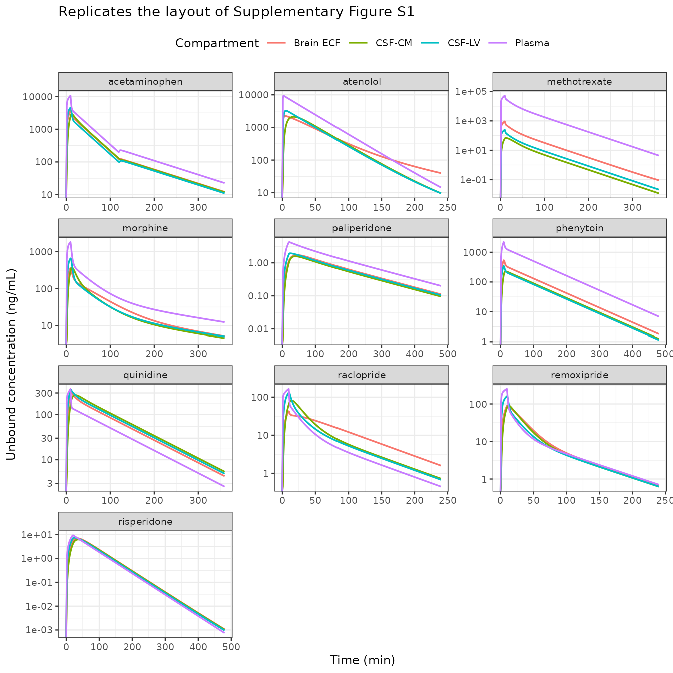
The ordering the paper emphasises is visible: for the efflux-transported compounds (atenolol, methotrexate, phenytoin) brain ECF sits well below plasma, while quinidine – the one compound with net active influx – sits above it.
Lysosomal trapping
The paper adds lysosomes specifically to capture trapping of basic
compounds. Because PHF7 is the uncharged fraction at
lysosomal pH 5.0 relative to plasma pH 7.4, a strong base accumulates
and a neutral compound does not.
lyso <- lapply(c("quinidine", "phenytoin"), function(d) {
  row <- dose_tab[dose_tab$drug == d, ]
  amt <- row$mgkg * BW * 1e6
  ev <- et(amt = amt, rate = amt / row$inf_min, cmt = "central")
  ev <- add.sampling(ev, seq(0, row$tmax_min, length.out = 200))
  s <- suppressWarnings(rxSolve(zeroRe(models[[d]]), ev, returnType = "data.frame"))
  tibble::tibble(time = s$time, drug = d,
                 `Brain ICF` = s$Cbrain_icf, `Brain ECF` = s$Cbrain_ecf)
}) |> bind_rows() |>
  pivot_longer(c(`Brain ICF`, `Brain ECF`), names_to = "Compartment", values_to = "conc")
#> ℹ omega/sigma items treated as zero: 'etalcl', 'etalq', 'etalvp'
#> ℹ omega/sigma items treated as zero: 'etalcl', 'etalvc'

ggplot(lyso, aes(time, conc, colour = Compartment)) +
  geom_line(linewidth = 0.7) +
  facet_wrap(~drug, scales = "free_y") +
  labs(x = "Time (min)", y = "Unbound concentration (ng/mL)") +
  theme_bw()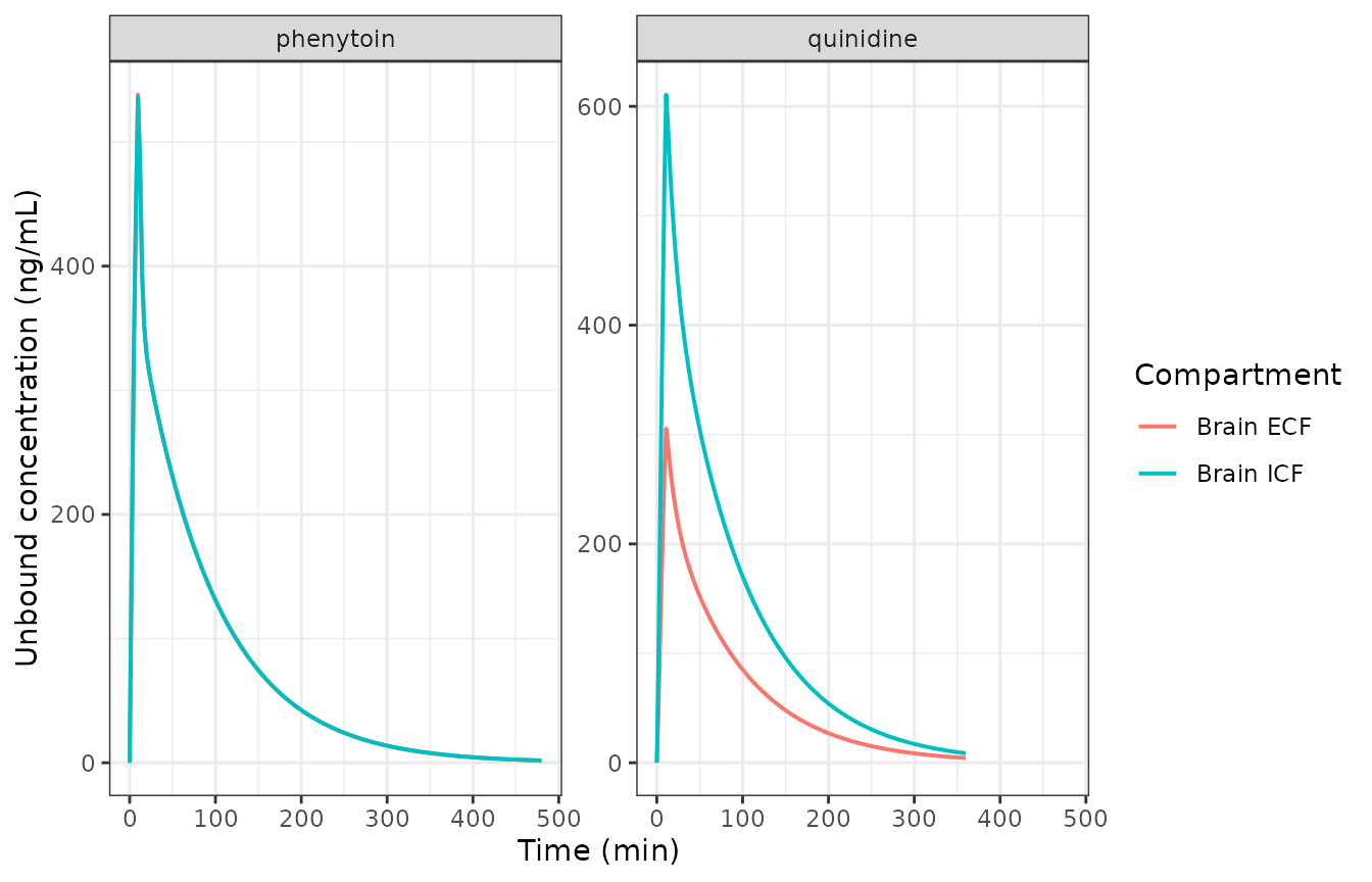
# Quinidine (base, pKa 9.1) concentrates intracellularly relative to ECF;
# phenytoin (neutral, PHF4 = PHF5 = 1) equilibrates 1:1. Structural, not
# stochastic -- a tight bound is correct here.
ratio <- lyso |>
  pivot_wider(names_from = Compartment, values_from = conc) |>
  filter(time > 120) |>
  group_by(drug) |>
  summarise(r = median(`Brain ICF` / `Brain ECF`), .groups = "drop")
stopifnot(
  ratio$r[ratio$drug == "phenytoin"] > 0.98,
  ratio$r[ratio$drug == "phenytoin"] < 1.02,
  # PHF4 / PHF5 = 0.80 / 0.40 = 2 for quinidine
  abs(ratio$r[ratio$drug == "quinidine"] - 2) < 0.05
)
ratio
#> # A tibble: 2 × 2
#>   drug          r
#>   <chr>     <dbl>
#> 1 phenytoin  1.00
#> 2 quinidine  2.00
Enterohepatic recirculation (acetaminophen)
Acetaminophen is the one drug with a thirteenth compartment: control stream S3 returns a fraction 0.693 of eliminated drug to plasma, switched on 120 min after the dose.
amt <- 15 * BW * 1e6
ev <- et(amt = amt, rate = amt / 10, cmt = "central")
ev <- add.sampling(ev, seq(0, 600, length.out = 400))
ehc <- suppressWarnings(rxSolve(zeroRe(models$acetaminophen), ev,
                                returnType = "data.frame"))
#> ℹ omega/sigma items treated as zero: 'etalvp'
ggplot(ehc, aes(time, Cc)) +
  geom_line(linewidth = 0.7) +
  geom_vline(xintercept = 120, linetype = 2, colour = "grey40") +
  scale_y_log10() +
  labs(x = "Time (min)", y = "Plasma concentration (ng/mL)",
       caption = "Dashed line: t_ehc = 120 min, when recirculation switches on") +
  theme_bw()
#> Warning in scale_y_log10(): log-10 transformation introduced infinite values.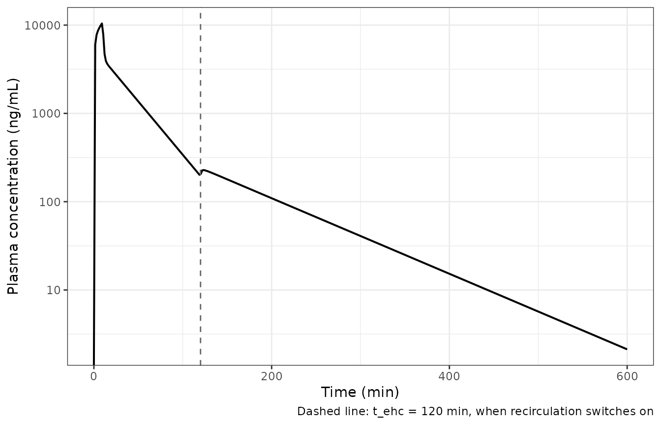
PKNCA validation
Plasma non-compartmental analysis on the simulated typical-value
profiles. Because the CNS subsystem is closed – every molecule that
crosses either barrier eventually returns to plasma through the
subarachnoid space – plasma AUC(0-inf) must equal
Dose / CL exactly. That is a real test of the
transcription: a sign error or a dropped return term anywhere in the
nine CNS ODEs would leak mass and break it.
Acetaminophen is the deliberate exception. Its enterohepatic
compartment gives the drug a second pass through plasma, so integrating
the mass balance gives AUC = Dose / (CL * (1 - F_ehc)) once
recirculation is active. Its AUC must therefore come out above
Dose / CL, and that excess is itself a check that the
recirculation term is wired up.
nca_one <- function(d) {
  row <- dose_tab[dose_tab$drug == d, ]
  amt <- row$mgkg * BW * 1e6
  ev <- et(amt = amt, rate = amt / row$inf_min, cmt = "central")
  # The tail runs to 3 x the plotting window, which is 10-20 terminal
  # half-lives for every drug here: far enough that the extrapolation to
  # infinity is negligible, but not so far that the solver's absolute
  # tolerance starts producing tiny negative concentrations (which make
  # PKNCA's log-trapezoidal rule return NaN).
  ev <- add.sampling(ev, sort(unique(c(
    0, seq(0, row$inf_min, length.out = 10),
    exp(seq(log(1), log(row$tmax_min * 3), length.out = 160))
  ))))
  pars <- if (d == "morphine") c(DOSE_HIGH = 0, OCC = 1) else NULL
  s <- suppressWarnings(rxSolve(zeroRe(models[[d]]), ev, params = pars,
                                returnType = "data.frame"))
  conc <- s |>
    filter(!is.na(Cc)) |>
    transmute(id = 1L, treatment = d, time = time, Cc = Cc)
  dosing <- data.frame(id = 1L, treatment = d, time = 0, dose = amt,
                       duration = row$inf_min)
  o_conc <- PKNCAconc(conc, Cc ~ time | treatment + id,
                      concu = "ng/mL", timeu = "min")
  o_dose <- PKNCAdose(dosing, dose ~ time | treatment + id,
                      duration = "duration", doseu = "ng")
  res <- pk.nca(PKNCAdata(
    o_conc, o_dose,
    intervals = data.frame(start = 0, end = Inf, auclast = TRUE,
                           aucinf.obs = TRUE, cmax = TRUE, tmax = TRUE,
                           half.life = TRUE)
  ))
  as.data.frame(res) |> mutate(treatment = d)
}

nca <- suppressWarnings(bind_rows(lapply(drugs, nca_one)))
#> ℹ omega/sigma items treated as zero: 'etalvp'
#> ℹ omega/sigma items treated as zero: 'etalcl', 'etalq2', 'etalvc'
#> ℹ omega/sigma items treated as zero: 'etalcl', 'etalq', 'etalq2', 'etalvc', 'etalvp', 'etaiov_1', 'etaiov_2'
#> ℹ omega/sigma items treated as zero: 'etalcl', 'etalvc'
#> ℹ omega/sigma items treated as zero: 'etalcl', 'etalvc'
#> ℹ omega/sigma items treated as zero: 'etalcl', 'etalq', 'etalvp'
#> ℹ omega/sigma items treated as zero: 'etalcl'
#> ℹ omega/sigma items treated as zero: 'etalcl', 'etalq', 'etalq2', 'etalvc'
#> ℹ omega/sigma items treated as zero: 'etalcl', 'etalvc'

nca_tab <- nca |>
  filter(PPTESTCD %in% c("cmax", "tmax", "aucinf.obs", "half.life")) |>
  select(treatment, PPTESTCD, PPORRES) |>
  pivot_wider(names_from = PPTESTCD, values_from = PPORRES) |>
  left_join(
    tibble::tibble(
      treatment = drugs,
      cl = vapply(models, function(m) exp(unname(m$theta["lcl"])), numeric(1)),
      dose = dose_tab$mgkg[match(drugs, dose_tab$drug)] * BW * 1e6
    ),
    by = "treatment"
  ) |>
  mutate(
    `Dose/CL` = dose / cl,
    `% diff` = 100 * (aucinf.obs - `Dose/CL`) / `Dose/CL`
  )

nca_tab |>
  mutate(across(c(cmax, tmax, aucinf.obs, half.life, `Dose/CL`), ~ signif(.x, 4)),
         `% diff` = round(`% diff`, 2)) |>
  select(treatment, cmax, tmax, half.life, aucinf.obs, `Dose/CL`, `% diff`) |>
  dplyr::rename("Drug" = treatment, "Cmax (ng/mL)" = cmax, "Tmax (min)" = tmax,
                "t1/2 (min)" = half.life,
                "AUC0-inf, NCA (ng*min/mL)" = aucinf.obs,
                "Dose/CL (ng*min/mL)" = `Dose/CL`) |>
knitr::kable()| Drug | Cmax (ng/mL) | Tmax (min) | t1/2 (min) | AUC0-inf, NCA (ng*min/mL) | Dose/CL (ng*min/mL) | % diff |
|---|---|---|---|---|---|---|
| acetaminophen | 10790.000 | 10 | 70.48 | 254300.0 | 237300.0 | 7.16 |
| atenolol | 9627.000 | 1 | 74.26 | 350600.0 | 350600.0 | 0.00 |
| methotrexate | 53350.000 | 10 | 214.60 | 1242000.0 | 1244000.0 | -0.13 |
| morphine | 1847.000 | 10 | 157.20 | 44240.0 | 44250.0 | -0.02 |
| paliperidone | 4.312 | 20 | 112.20 | 637.8 | 637.8 | 0.00 |
| phenytoin | 2254.000 | 10 | 61.29 | 138900.0 | 138900.0 | 0.00 |
| quinidine | 374.600 | 10 | 60.20 | 15410.0 | 15430.0 | -0.12 |
| raclopride | 166.800 | 10 | 47.83 | 3000.0 | 3017.0 | -0.57 |
| remoxipride | 254.700 | 10 | 51.36 | 4138.0 | 4147.0 | -0.23 |
| risperidone | 9.511 | 20 | 34.09 | 564.3 | 564.3 | 0.00 |
closed <- nca_tab[nca_tab$treatment != "acetaminophen", ]
ehc_row <- nca_tab[nca_tab$treatment == "acetaminophen", ]
stopifnot(
  # The nine drugs with a single elimination path: AUC must equal Dose / CL.
  # Trapezoidal AUC on a log-spaced grid, so allow a little numerical slack,
  # but no drug may leak out of the CNS subsystem.
  max(abs(closed$`% diff`)) < 2,
  median(abs(closed$`% diff`)) < 1,
  # Acetaminophen must sit above Dose / CL because 69.3 % of eliminated drug is
  # returned to plasma after 120 min, and below the 226 % excess that would
  # result if recirculation were active from time zero.
  ehc_row$`% diff` > 2,
  ehc_row$`% diff` < 226
)
The paper reports no non-compartmental summaries of its own, so there is no published NCA table to compare against; the comparison above is the internal mass-balance check.
A stochastic cohort
Quinidine carries interindividual variability on clearance, intercompartmental clearance and peripheral volume (Table 2). 100 animals, well inside the 200-per-arm cap.
rxSetSeed(20171011)
amt <- 10 * BW * 1e6
ev <- et(amt = amt, rate = amt / 10, cmt = "central")
ev <- add.sampling(ev, seq(0, 360, length.out = 120))
sim <- suppressWarnings(rxSolve(models$quinidine, ev, nSub = 100,
                                returnType = "data.frame"))

sim |>
  select(sim.id, time, Plasma = Cc, `Brain ECF` = Cbrain_ecf,
         `Total brain` = Cbrain_total) |>
  pivot_longer(-c(sim.id, time), names_to = "Compartment", values_to = "conc") |>
  group_by(Compartment, time) |>
  summarise(med = median(conc), lo = quantile(conc, 0.05),
            hi = quantile(conc, 0.95), .groups = "drop") |>
  ggplot(aes(time, med, colour = Compartment, fill = Compartment)) +
  geom_ribbon(aes(ymin = lo, ymax = hi), alpha = 0.18, colour = NA) +
  geom_line(linewidth = 0.7) +
  scale_y_log10() +
  labs(x = "Time (min)", y = "Concentration (ng/mL)",
       title = "Quinidine 10 mg/kg, 100 simulated rats (median, 5th-95th percentile)") +
  theme_bw()
#> Warning in scale_y_log10(): log-10 transformation introduced infinite values.
#> log-10 transformation introduced infinite values.
#> log-10 transformation introduced infinite values.
#> log-10 transformation introduced infinite values.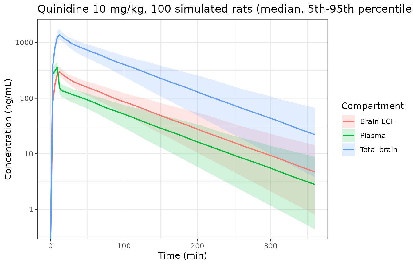
# Structural ordering that must hold for every animal at every time after the
# infusion: total brain > brain ECF for quinidine, because the binding factor
# (7.2) and the lysosomal / intracellular pools all add to the total.
late <- sim[sim$time > 60, ]
stopifnot(all(late$Cbrain_total > late$Cbrain_ecf))
Assumptions and deviations
Ten files, one structure. The authors published one generic CNS model and eleven control streams. Each drug becomes one model file, following the same shape as the
Saleh_2023_*_mouse_pbpkfamily. Morphine’s two control streams (S6 for 4 mg/kg, S7 for 10 and 40 mg/kg) are a single file with aDOSE_HIGHcovariate, because Table 4 presents them as one drug with dose-stratified footnotes a and b.Plasma parameters are taken from Table 2, not from the control streams. The two agree exactly for nine of the ten drugs – including which parameters carry interindividual variability, and with
$OMEGAequal to the square of the tabulated coefficient of variation in every case. See Errata for atenolol.The binding factor
BFdoes not affect the ODE solution. The control streams defineC4 = A(4)/V4*BFand then useC4/BFat every occurrence in$DES, soBFcancels; it survives only in the total-brain output. This implementation uses the unbound concentration directly in the ODEs and appliesBFonly inCbrain_total, which is algebraically identical and makes the cancellation explicit.Cbrain_totalis provided for nine drugs, not three. The authors coded the total-brain output only in the three control streams that had total-brain data to compare against (quinidine, raclopride, remoxipride). BecauseBFis published in Table 5 for nine drugs, the same expression is emitted for all nine; methotrexate hasKp= NA andBF= NA and gets no total-brain output. Only the three the authors plotted were validated against data.Rat body weight. Table 1 gives doses in mg/kg while every volume and flow in Table 3 is absolute. This vignette uses 0.25 kg, the midpoint of the 225-275 g range in Supplementary Material S2, to convert. The model files themselves take an absolute amount in ng and are weight-agnostic.
Kp,uuis relative to total plasma concentration. The model drives barrier transport from the microvascular concentration, which equals the total plasma concentration at steady state – unbound fraction in plasma never enters the ODEs. Table 4’sKp,uuvalues are reproduced on that basis (Validation 2), so the paper’sfu,pcolumn is descriptive only and is not encoded.Equations 1 and 2 are not re-derived. The molecular-weight and logP regressions for
DaqandP0are reproduced verbatim only in references 16 and 17, which were not available when this model was built. The tabulated per-drug values of Table 4 are encoded directly instead. (They are self-consistent: evaluatingDaq = 10^(-4.113 - 0.4609*log10(MW)) * 60andP0 = 10^(0.939*logP - 6.21) * 60, the forms the sibling LeiCNS mouse papers publish, returns every tabulated value for all ten drugs.)
Errata and unresolved inconsistencies in the source
Atenolol, Table 2 versus control stream S4. Table 2 reports
V_PL= 256 mL and no interindividual variability at all; S4 carriesTHETA(10)= 259 and$OMEGA= 0.02 (a 14.1 % coefficient of variation) onV1. Table 2 is used here, because it is the paper’s reported final parameter table and it agrees exactly with the control stream for the other nine drugs, and because an$OMEGAof exactly 0.02 has the signature of a leftover initial estimate – two sibling streams still carry explicit; initial estimatescomments. Atenolol is therefore a typical-value-only plasma model here.Methotrexate
AFout2. Control stream S5 setsAF22= 46353.1. That is contradicted by three independent readings in the paper: Table 4 printsAFout2= 4.7 x 10^5, Table 5 printsQBCSFB1_out= 2.2 mL/min (which requiresAFout2near 4.4 x 10^5), and the reportedKp,uu,CSFLV= 0.0066 requires roughly 3.4 x 10^5. The control-stream value would giveQBCSFB1_out= 0.24 mL/min, an order of magnitude out. It reads as a misplaced decimal point, so Table 4’s 4.7 x 10^5 is used. The two other methotrexate efflux factors,AFout1andAFout3, are taken from the control stream because they agree with Table 4.Table 5 cells contradicted by their own row. Four of the 160 published combined clearances do not follow from Table 5’s own components via Table 5’s own footnote formulas: quinidine
QBBB_out,QBCSFB1_outandQBCSFB2_out, and racloprideQBCSFB1_in. Details under Validation 1. The primitives are encoded, so this implementation follows the formulas.CSF
Kp,uudoes not close as tightly as brain-ECFKp,uu. Running the published model to steady state returns Table 4’sKp,uu,brainECFwithin 6 % for all ten drugs, but the CSF ratios within 10 % for only eight of ten: phenytoin (0.16 predicted versus 0.26 published), quinidine (1.72 versus 1.5) and methotrexate CSF-LV (0.0048 versus 0.0066) deviate. The asymmetry factors are inputs to the simulation and were reproduced from Table 4, and the derived clearances reproduce Table 5 (Validation 1), so this is a property of the paper’s own back-solution ofAFin2/AFout2andAFin3/AFout3rather than of the transcription. The size of the deviation tracks how transcellular the blood-CSF barrier clearance is for that compound, which is what an error in a transcellular-only asymmetry factor would do. The closed forms in Supplementary Material S1 could not be evaluated independently: the supplement is a Word document whose equation rendering has lost its fraction structure, so numerator and denominator terms are run together. Anyone depending on absolute CSF predictions for these three compounds should treat them accordingly.The binding factor does not reproduce Table 4’s
Kp. Solving the coded total-brain expression at steady state impliesKpnear 7.0 for quinidine, 5.4 for raclopride and 3.4 for remoxipride, against the 13, 11 and 5.5 printed in Table 4.BFis nonetheless unambiguous – Table 5 and the control streams give the same values (7.2, 8.5, 5.3) – so it is encoded as published. The same Supplementary Material S1 rendering problem prevents checking the authors’BFderivation.An undocumented morphine covariate is left at its reference level. Control streams S6 and S7 multiply plasma clearance by
THETA(13)= 1.08 when a data columnBLOCKequals 1.BLOCKis defined nowhere in the paper, its supplement or Table 2, and Table 2 does not report the coefficient. The extraction uses the reference level (BLOCK= 0, factor 1), which is what Table 2 describes.Author-line correction. The article carries a publisher notice: it was published online 13 October 2017, an error in the author line was identified, and the corrected version was posted 27 October 2017. The correction does not touch any model value.