TF-505 (Matsumoto 2005)
Source:vignettes/articles/Matsumoto_2005_TF_505.Rmd
Matsumoto_2005_TF_505.RmdModel and source
- Citation: Matsumoto Y, Fujita T, Ishida Y, Shimizu M, Kakuo H, Yamashita K, Majima M, Kumagai Y. Population Pharmacokinetic-Pharmacodynamic Modeling of TF-505 Using Extension of Indirect Response Model by Incorporating a Circadian Rhythm in Healthy Volunteers. Biol Pharm Bull. 2005;28(8):1455-1461. doi:10.1248/bpb.28.1455
- Description: Two-compartment first-order-absorption population PK model for the oral 5-alpha-reductase inhibitor TF-505 coupled to an indirect-response PD model for plasma dihydrotestosterone (DHT, expressed as percent of basal) in which the DHT synthesis rate kin is modulated by a 24-h circadian cosine; fit to single- and multiple-dose data from healthy adult male Japanese volunteers (Matsumoto 2005).
- Article: Biol Pharm Bull. 2005;28(8):1455-1461
Population
The study enrolled 36 healthy adult male Japanese volunteers, divided into six dose groups of six subjects each (Matsumoto 2005 Table 1). The first four groups received single oral doses of TF-505 (25, 50, 75 or 100 mg) at 9 a.m. without breakfast. The two remaining groups received repeated oral doses (12.5 or 25 mg) once daily for 7 days at 9 a.m. after breakfast. Inclusion required age >=20 years (for the low single-dose groups 25 and 50 mg) or >=40 years (for the high single-dose 75 / 100 mg groups and both multiple-dose groups), and body weight within 20% of ideal. Group mean ages ranged 22.8-52.5 years (overall span 20-64 y) and group mean weights ranged 61.1-65.7 kg (overall span 49.6-72.3 kg).
The population metadata is available programmatically:
rxode2::rxode(readModelDb("Matsumoto_2005_TF_505"))$meta$population
#> ℹ parameter labels from comments will be replaced by 'label()'
#> $species
#> [1] "human"
#>
#> $n_subjects
#> [1] 36
#>
#> $n_studies
#> [1] 1
#>
#> $age_range
#> [1] "20-64 years"
#>
#> $age_median
#> NULL
#>
#> $weight_range
#> [1] "49.6-72.3 kg"
#>
#> $weight_median
#> NULL
#>
#> $sex_female_pct
#> [1] 0
#>
#> $race_ethnicity
#> Japanese
#>      100
#>
#> $disease_state
#> [1] "Healthy adult male Japanese volunteers"
#>
#> $dose_range
#> [1] "Single 25, 50, 75, 100 mg p.o.; multiple 12.5 or 25 mg p.o. QD x 7 days"
#>
#> $regions
#> [1] "Japan"
#>
#> $notes
#> [1] "Inclusion: males aged >=20 years (low single-dose groups 25 and 50 mg) or >=40 years (high single-dose 75 / 100 mg, and both multiple-dose groups); body weight within 20% of ideal. Single-dose groups dosed at 9 a.m. without breakfast; multiple-dose groups dosed at 9 a.m. after breakfast. Smoking allowed but stopped 1 h pre- through 24 h post-dose. Caffeine, alcohol and grapefruit prohibited. 564 plasma TF-505 and 264 plasma DHT measurements were used in the joint fit."
Source trace
The per-parameter origin is recorded as an in-file comment next to
each ini() entry in
inst/modeldb/specificDrugs/Matsumoto_2005_TF_505.R. The
table below collects them in one place.
| Equation / parameter | Value | Source location |
|---|---|---|
| Two-compartment PK with first-order absorption | n/a | Matsumoto 2005 Results ‘Pharmacokinetic and Pharmacodynamic Model’ (PK Model 2 in Table 2 was selected) |
| Indirect-response PD on DHT with inhibition of input | n/a | Matsumoto 2005 Eq. (1) |
| Circadian kin = Rm + Ramp * cos(2pi(t - Tz)/24) | n/a | Matsumoto 2005 Eq. (2); PD Model 5 in Table 3 was selected |
| ka | 0.197 1/h | Table 4 |
| ke | 0.0678 1/h | Table 4 (reparameterised to lcl = log(ke*Vc)) |
| Vc | 12.5 L | Table 4 |
| k12 | 0.0645 1/h | Table 4 |
| k21 | 0.0723 1/h | Table 4 |
| IC50 | 1.01 ug/mL | Table 4 |
| kout | 0.221 1/h | Table 4 |
| Rm | 20.4 %/h | Table 4 |
| Ramp | 5.06 %/h | Table 4 |
| Tz (acrophase) | 5.01 h | Table 4 |
| Imax | 0.706 | Table 4 |
| IIV omega^2 (ka, ke, Vc, k12, kout, Rm, Tz, Imax) | various | Table 4 ‘Inter-individual variability’ column (k21, IC50, Ramp fixed at 0 per footnote a) |
| Residual sigma^2 (PK 0.191, PD 0.0419) | n/a | Table 4 ‘Intra-individual residual variability’ (CV per text: 43.70% PK, 20.47% PD) |
Virtual cohort
The vignette uses small virtual cohorts (50 subjects per dose group) that mirror the trial’s single-dose arms (25, 50, 75 and 100 mg p.o.). The trial recruited Japanese male volunteers in tight body-weight and age ranges and the published popPK / popPD model carries no covariate effects, so the cohort needs no demographic columns.
set.seed(723)

make_single_dose_cohort <- function(n, dose_mg, id_offset = 0L) {
  # one dosing row + a 73-point observation grid (0-72 h post-dose)
  ids <- id_offset + seq_len(n)
  obs_grid <- seq(0, 72, by = 1)
  dose <- tibble(
    id   = ids,
    time = 0,
    amt  = dose_mg,
    rate = 0,
    cmt  = "depot",
    evid = 1L,
    dose_group = sprintf("%g mg", dose_mg)
  )
  obs <- tidyr::expand_grid(
    id = ids,
    time = obs_grid
  ) |>
    mutate(
      amt  = 0,
      rate = 0,
      cmt  = "Cc",
      evid = 0L,
      dose_group = sprintf("%g mg", dose_mg)
    )
  bind_rows(dose, obs) |>
    arrange(id, time, desc(evid))
}

dose_levels <- c(25, 50, 75, 100)
events_sd <- bind_rows(lapply(seq_along(dose_levels), function(i) {
  make_single_dose_cohort(n = 50L, dose_mg = dose_levels[i],
                          id_offset = (i - 1L) * 50L)
}))

stopifnot(!anyDuplicated(unique(events_sd[, c("id", "time", "evid")])))
Simulation - single doses
mod <- rxode2::rxode(readModelDb("Matsumoto_2005_TF_505"))
#> ℹ parameter labels from comments will be replaced by 'label()'

sim_sd <- rxode2::rxSolve(
  mod,
  events = events_sd,
  keep   = "dose_group",
  returnType = "data.frame"
) |>
  mutate(dose_group = factor(dose_group,
                             levels = sprintf("%g mg", dose_levels)))
Replicate Figure 2 - single-dose TF-505 plasma concentration
sim_sd_summary <- sim_sd |>
group_by(dose_group, time) |>
summarise(
Q05 = quantile(Cc, 0.05, na.rm = TRUE),
Q50 = quantile(Cc, 0.50, na.rm = TRUE),
Q95 = quantile(Cc, 0.95, na.rm = TRUE),
.groups = "drop"
)
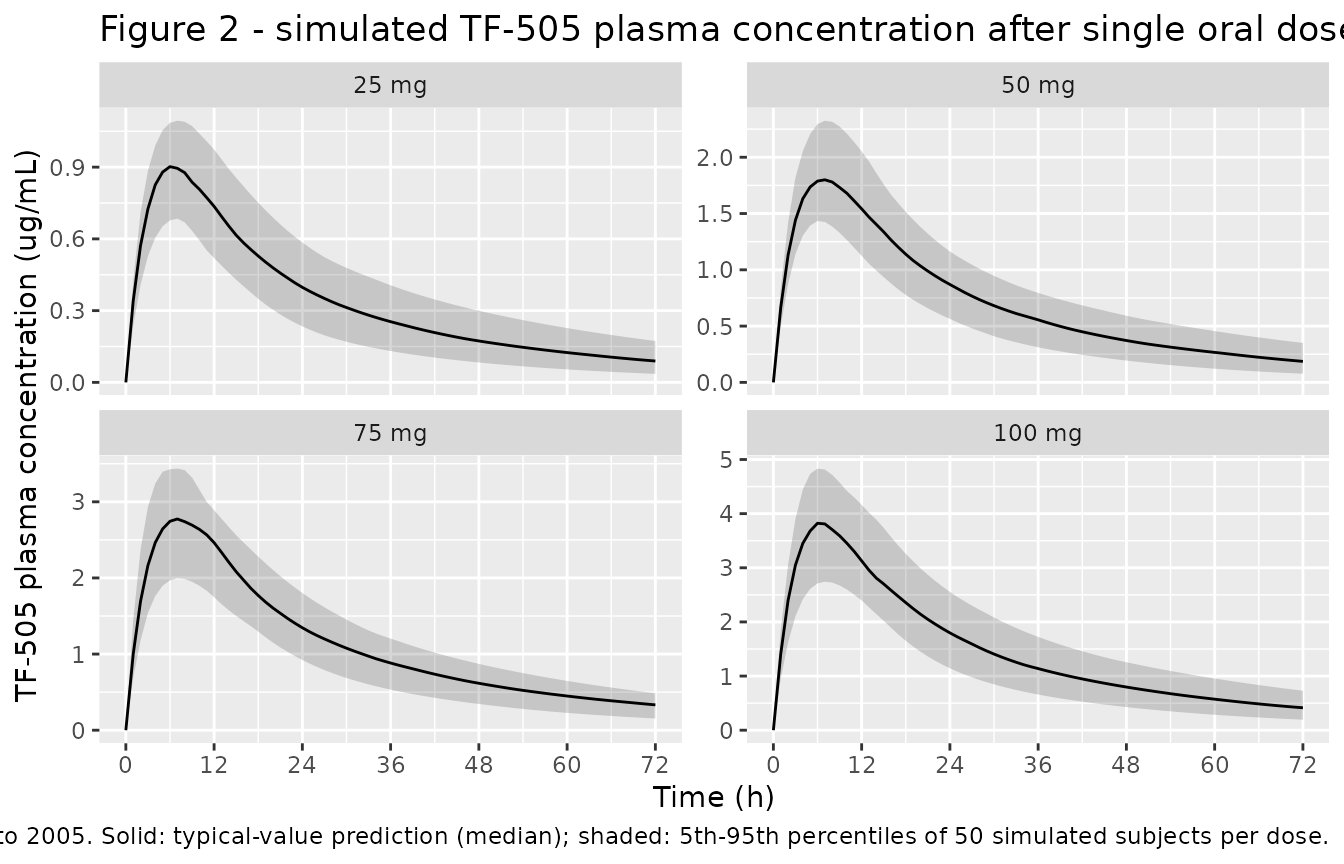
ggplot(sim_sd_summary, aes(time, Q50)) +
geom_ribbon(aes(ymin = Q05, ymax = Q95), alpha = 0.20) +
geom_line() +
facet_wrap(~dose_group, scales = "free_y") +
scale_x_continuous(breaks = seq(0, 72, by = 12)) +
labs(
x = "Time (h)",
y = "TF-505 plasma concentration (ug/mL)",
title = "Figure 2 - simulated TF-505 plasma concentration after single oral doses",
caption = "Replicates Figure 2 of Matsumoto 2005. Solid: typical-value prediction (median); shaded: 5th-95th percentiles of 50 simulated subjects per dose."
)
Replicate Figure 6 - single-dose plasma DHT (% basal)
sim_sd_dht <- sim_sd |>
group_by(dose_group, time) |>
summarise(
Q05 = quantile(DHT, 0.05, na.rm = TRUE),
Q50 = quantile(DHT, 0.50, na.rm = TRUE),
Q95 = quantile(DHT, 0.95, na.rm = TRUE),
.groups = "drop"
)
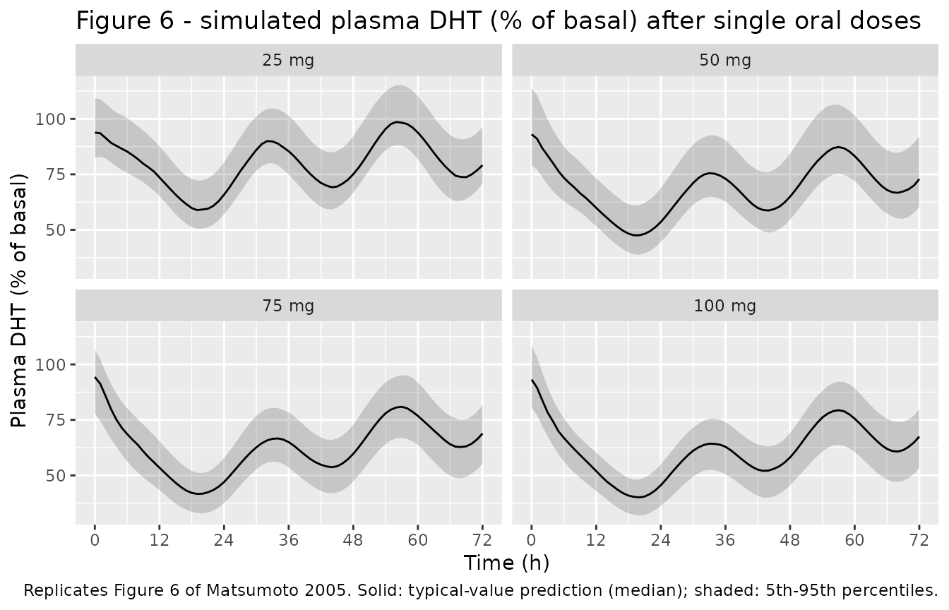
ggplot(sim_sd_dht, aes(time, Q50)) +
geom_ribbon(aes(ymin = Q05, ymax = Q95), alpha = 0.20) +
geom_line() +
facet_wrap(~dose_group) +
scale_x_continuous(breaks = seq(0, 72, by = 12)) +
labs(
x = "Time (h)",
y = "Plasma DHT (% of basal)",
title = "Figure 6 - simulated plasma DHT (% of basal) after single oral doses",
caption = "Replicates Figure 6 of Matsumoto 2005. Solid: typical-value prediction (median); shaded: 5th-95th percentiles."
)
Replicate Figure 3 - multiple-dose TF-505 plasma concentration
make_multidose_cohort <- function(n, dose_mg, n_doses = 7L, dose_interval_h = 24,
                                  obs_end = 192, id_offset = 0L) {
  ids <- id_offset + seq_len(n)
  dose_times <- (seq_len(n_doses) - 1L) * dose_interval_h
  doses <- tidyr::expand_grid(id = ids, time = dose_times) |>
    mutate(
      amt  = dose_mg,
      rate = 0,
      cmt  = "depot",
      evid = 1L,
      dose_group = sprintf("%g mg QD x %d", dose_mg, n_doses)
    )
  obs <- tidyr::expand_grid(
    id = ids,
    time = seq(0, obs_end, by = 2)
  ) |>
    mutate(
      amt  = 0,
      rate = 0,
      cmt  = "Cc",
      evid = 0L,
      dose_group = sprintf("%g mg QD x %d", dose_mg, n_doses)
    )
  bind_rows(doses, obs) |>
    arrange(id, time, desc(evid))
}

md_levels <- c(12.5, 25)
events_md <- bind_rows(lapply(seq_along(md_levels), function(i) {
  make_multidose_cohort(n = 50L, dose_mg = md_levels[i],
                        id_offset = 1000L + (i - 1L) * 50L)
}))

sim_md <- rxode2::rxSolve(
  mod,
  events = events_md,
  keep   = "dose_group",
  returnType = "data.frame"
) |>
  mutate(dose_group = factor(dose_group,
                             levels = sprintf("%g mg QD x %d", md_levels, 7L)))

sim_md_summary <- sim_md |>
  group_by(dose_group, time) |>
  summarise(
    Q05 = quantile(Cc, 0.05, na.rm = TRUE),
    Q50 = quantile(Cc, 0.50, na.rm = TRUE),
    Q95 = quantile(Cc, 0.95, na.rm = TRUE),
    .groups = "drop"
  )

ggplot(sim_md_summary, aes(time, Q50)) +
  geom_ribbon(aes(ymin = Q05, ymax = Q95), alpha = 0.20) +
  geom_line() +
  facet_wrap(~dose_group) +
  scale_x_continuous(breaks = seq(0, 192, by = 24)) +
  labs(
    x = "Time (h)",
    y = "TF-505 plasma concentration (ug/mL)",
    title = "Figure 3 - simulated TF-505 plasma concentration after repeated daily oral doses",
    caption = "Replicates Figure 3 of Matsumoto 2005. Solid: median; shaded: 5th-95th percentiles of 50 simulated subjects per dose. Each subject receives once-daily dosing for 7 consecutive days at t = 0, 24, 48, 72, 96, 120, 144 h."
  )
PKNCA validation
The paper reports preliminary NCA for the single-dose arms (Matsumoto 2005 Results ‘Pharmacokinetic and Pharmacodynamic Model’ paragraph 1): Tmax, Cmax and AUC0-72. We run PKNCA on the simulated single-dose cohorts and compare against the published values.
sim_nca <- sim_sd |>
  filter(!is.na(Cc), time > 0 | time == 0) |>
  select(id, time, Cc, dose_group)

conc_obj <- PKNCA::PKNCAconc(sim_nca, Cc ~ time | dose_group + id)

dose_df <- events_sd |>
  filter(evid == 1L) |>
  select(id, time, amt, dose_group)

dose_obj <- PKNCA::PKNCAdose(dose_df, amt ~ time | dose_group + id)

intervals <- data.frame(
  start      = 0,
  end        = 72,
  cmax       = TRUE,
  tmax       = TRUE,
  auclast    = TRUE
)

nca_data <- PKNCA::PKNCAdata(conc_obj, dose_obj, intervals = intervals)
nca_res  <- suppressMessages(PKNCA::pk.nca(nca_data))

nca_tbl <- as.data.frame(nca_res$result) |>
  filter(PPTESTCD %in% c("cmax", "tmax", "auclast")) |>
  group_by(dose_group, PPTESTCD) |>
  summarise(mean = mean(PPORRES, na.rm = TRUE),
            sd   = sd(PPORRES, na.rm = TRUE),
            .groups = "drop") |>
  mutate(value = sprintf("%.2f \U00B1 %.2f", mean, sd)) |>
  select(dose_group, PPTESTCD, value) |>
  tidyr::pivot_wider(names_from = PPTESTCD, values_from = value)

knitr::kable(
  nca_tbl,
  caption = "Simulated single-dose NCA parameters by dose group (mean +/- SD over 50 virtual subjects)."
)| dose_group | auclast | cmax | tmax |
|---|---|---|---|
| 100 mg | 109.38 ± 25.03 | 3.79 ± 0.68 | 6.80 ± 0.73 |
| 25 mg | 25.10 ± 5.65 | 0.90 ± 0.13 | 6.60 ± 0.78 |
| 50 mg | 53.12 ± 11.20 | 1.83 ± 0.28 | 6.80 ± 0.73 |
| 75 mg | 82.05 ± 16.70 | 2.80 ± 0.52 | 6.94 ± 0.84 |
Comparison against published NCA
The simulated values can be compared row-by-row against the published values (Matsumoto 2005 Results paragraph 1):
| Dose | Cmax (paper, ug/mL) | Tmax (paper, h) | AUC0-72 (paper, ug.h/mL) |
|---|---|---|---|
| 25 mg | 1.10 +/- 0.38 | 4.38 +/- 1.01 | 32.12 +/- 14.46 |
| 50 mg | 2.45 +/- 0.70 | 5.47 +/- 2.34 | 76.95 +/- 15.96 |
| 75 mg | 3.79 +/- 1.92 | 4.23 +/- 0.86 | 97.50 +/- 46.82 |
| 100 mg | 3.12 +/- 1.20 | 3.85 +/- 0.73 | 73.22 +/- 26.74 |
The paper notes (Results paragraph 1) that the 100 mg dose exhibits saturable absorption relative to lower doses, producing lower Cmax and AUC than expected from linear dose scaling. The packaged model is a purely linear two-compartment PK model with first-order absorption (the published final PK model; saturable Michaelis-Menten absorption was a candidate in PK Model 3 / 4 in Table 2 but was not selected), so the simulation predicts dose-proportional Cmax and AUC. Reviewers comparing simulated and observed values for the 100 mg arm should expect the simulation to over-predict Cmax / AUC at 100 mg by the proportion corresponding to the saturable-absorption observation in the data. This is the model’s intended behaviour, not a translation error.
Assumptions and deviations
-
Reparameterisation from micro-rate-constants to canonical CL
/ Vc / Q / Vp form. Matsumoto 2005 reports PK parameters as the
micro-rate constants
ka,ke,Vc,k12,k21. The packaged model reparameterises to the nlmixr2lib canonicallcl,lvc,lk12,lk21primaries (withkel = cl / vcrecovered insidemodel()). Typical-value predictions are exact:CL_pop = ke_pop * Vc_pop = 0.0678 * 12.5 = 0.8475 L/h. To preserve the paper’s underlying log-normal IIV structure on the original primaries (eta_ke,eta_Vcindependent per Methods ‘Pharmacostatistical Models’), the canonical encoding uses a 2x2 covariance block on(etalcl, etalvc)withvar(etalcl) = var(eta_ke) + var(eta_Vc) = 0.0481 + 0.0180 = 0.0661,cov(etalcl, etalvc) = var(eta_Vc) = 0.0180,var(etalvc) = 0.0180. This block is positive-definite (determinant 8.66e-4) and reproduces every marginal CV in Table 4 exactly:CV(CL) = sqrt(exp(0.0661) - 1) = 26.13%,CV(Vc) = sqrt(exp(0.0180) - 1) = 13.48%,CV(kel = CL/Vc) = sqrt(exp(var(etalcl) - 2*cov + var(etalvc)) - 1) = sqrt(exp(0.0481) - 1) = 22.20%(paper text: 21.93%, matches within rounding). - k21, IC50, Ramp IIVs fixed at zero. Matsumoto 2005 Table 4 footnote a notes ‘Fixed at zero due to small variance estimates’ for these three parameters in preliminary analysis (<10^-8). The packaged model encodes them as fixed-effect parameters with no associated eta term.
-
Initial DHT condition. The paper expresses DHT data
as a percent of basal; the no-drug steady-state of the model is
Rm / kout = 20.4 / 0.221 = 92.31%. The packaged model initialisesdht(0) = rm / koutso the simulation starts in (non-circadian) quasi-steady state. The circadian oscillation is established by the ODE within the first ~10-15 h. Users who prefer to start at the by-definition100%can passinits = c(dht = 100)torxSolve(); the model converges to the same circadian limit cycle either way. -
Acrophase Tz IIV on log scale. Matsumoto 2005
Methods states all PK and PD IIVs are log-normal, including the
acrophase Tz. The canonical
ltacro(log-transformed acrophase) preserves this encoding directly. The 8.37% reported CV on Tz translates to omega^2 = log(1 + 0.0837^2) = 0.00700 on the log scale, matching Table 4. - Saturable absorption at 100 mg not encoded. The paper notes (Results paragraph 1; Discussion) that the 100 mg dose appears to show saturation of absorption (lower observed Cmax / AUC than the linear dose-extrapolation prediction). The final PK model selected (PK Model 2 in Table 2) is linear; the candidate Michaelis-Menten absorption models (PK Models 3 and 4) had similar OFV but were not selected. The packaged model reproduces the published final PK model, so the simulation will over-predict 100 mg Cmax / AUC by the fraction corresponding to this saturation.
-
No covariates retained. Matsumoto 2005 does not
include any covariate effects in the final PK or PD model. The package
covariateDatalist is therefore empty. -
DHT ‘paper-specific’ compartment. The
dhtstate is declared viapaper_specific_compartmentssince it is a paper-mechanistic biomarker state without a canonical equivalent (analogous tonefainAhlstrom_2010_nicotinicAcid_rat, which is registered separately inR/conventions.R).