Intraperitoneal irinotecan and SN-38 (Rietveld 2024)
Source:vignettes/articles/Rietveld_2024_irinotecan.Rmd
Rietveld_2024_irinotecan.RmdModel and source
- Citation: Rietveld PCS, Sassen SDT, Guchelaar NAD, van Eerden RAG, de Boer NL, van den Heuvel TBM, Burger JWA, Mathijssen RHJ, Koch BCP, Koolen SLW. Population pharmacokinetics of intraperitoneal irinotecan and SN-38 in patients with peritoneal metastases from colorectal origin. CPT Pharmacometrics Syst Pharmacol. 2024;13(6):1006-1016. doi:10.1002/psp4.13136.
- Article (open access): https://doi.org/10.1002/psp4.13136
- PubMed Central: https://www.ncbi.nlm.nih.gov/pmc/articles/PMC11179701/
- Trial: INTERACT phase I (IP irinotecan with systemic FOLFOX-bevacizumab)
mod <- rxode2::rxode(readModelDb("Rietveld_2024_irinotecan"))
#> ℹ parameter labels from comments will be replaced by 'label()'
Population
Rietveld 2024 developed the model from the INTERACT phase I trial: 18 adults with extensive peritoneal metastases (Peritoneal Cancer Index > 20, median 29) from histologically proven colorectal cancer, all ineligible for cytoreductive surgery with hyperthermic intraperitoneal chemotherapy. Irinotecan 50 mg (n = 4), 75 mg (n = 9) or 100 mg (n = 5) was instilled into the peritoneal cavity over 1.5 h every two weeks through a peritoneal access port, concurrently with systemic FOLFOX plus bevacizumab. Ascites was drained before each instillation. The maximum tolerated dose was 75 mg two-weekly.
Baseline characteristics (paper Table 1): age median 64 years (42-77), weight median 79.7 kg (59-105), height median 177 cm (163-192), BSA median 1.97 m^2 (1.65-2.33), BMI median 26.9 kg/m^2 (20.9-31.8), 6 of 18 female, ECOG 0 (n = 12) or 1 (n = 6).
Samples used in the fit (paper Results): irinotecan in plasma (334), SN-38 in plasma (258) and SN-38 in peritoneal fluid (263), 855 in total. Note that IP irinotecan itself was never assayed – peritoneal samples were withdrawn through the same port used for the instillation, so measuring IP irinotecan would have been biased. Data from the first two cycles were pooled as time after dose; no accumulation was seen.
The same information is available programmatically via
rxode2::rxode(readModelDb("Rietveld_2024_irinotecan"))$population.
Structural model
The final model (paper Figure 1) has five compartments:
                       Ka2                        CL_M
      depot_ip_sn38  -------->  central_sn38  --------->
        (V5, 487 L)               (V4)
            ^                        ^
            | CLPM                   | MR * CL
            |                        |
 Dose -> depot_ip     -------->   central      --------->  (1 - MR) * CL
                        Ka          (V2)
                                     |  Q
                                     v
                                peripheral1
                                     (V3)
Irinotecan instilled into the peritoneal cavity
(depot_ip) leaves it by two parallel first-order routes:
absorption into plasma (ka_ip) and in-situ conversion to
SN-38 by peritoneal carboxylesterases (kmet_ip). A fixed
fraction fm = 3% of the irinotecan cleared from plasma
appears as SN-38 in plasma; the remainder is eliminated. The peritoneal
SN-38 pool (depot_ip_sn38) is absorbed into SN-38 plasma
with clearance Ka2 out of the fixed volume
V5.
Concentrations in the source are molar (paper Figure 4 plots
Log(nM)), so parent-to-metabolite transfer is
equimolar and no molecular-weight factor appears in the
model. Doses below are converted from mg to umol with the irinotecan
free-base molecular weight.
MW_IRI <- 586.68  # g/mol, irinotecan free base
MW_SN  <- 392.40  # g/mol, SN-38

# Covariate quantiles printed in the Figure 2 and Figure 3 legends.
WT_REF  <- 83.4   # kg,  Equation 2 normalising median
GGT_REF <- 32     # U/L, Equation 3 normalising median

doses_mg <- c(50, 75, 100)
dose_umol <- doses_mg / MW_IRI * 1000
names(dose_umol) <- paste(doses_mg, "mg")
round(dose_umol, 1)
#>  50 mg  75 mg 100 mg
#>   85.2  127.8  170.5
Source trace
Every ini() entry carries an in-file comment naming its
source row. The table below is the same provenance in one place.
| Parameter | Value | Source location |
|---|---|---|
| lka_ip | 1.02 1/h | Table 2, row Ka (RSE 9%) |
| fm | 0.03 FIX | Table 2, row MR; Results: fixed at 3% from literature |
| lcl | 33.2 L/h | Table 2, row CL (RSE 6%) |
| lvc | 225 L | Table 2, row V2 (RSE 11%) |
| lq | 13.9 L/h | Table 2, row Q (RSE 17%) |
| lvp | 119 L | Table 2, row V3 (RSE 14%) |
| lvc_sn38 | 15.9 L | Table 2, row V4 (RSE 26%) |
| lcl_sn38 | 46 L/h | Table 2, row CL_M (RSE 12%) |
| lkmet_ip | 0.118 1/h | Table 2, row CL_PM (RSE 14%) |
| lq_ip_sn38 | 4.68 L/h | Table 2, row Ka2 (RSE 15%) |
| lv_ip_sn38 | 487 L FIX | Table 2, row V5; fixed for covariance with CL_PM |
| e_wt_vc_sn38 | 5.31 | Table 2, Covariates row WT; Equation 2, (WT/83.4)^theta |
| e_ggt_cl_sn38 | -0.26 | Table 2, Covariates row GGT; Equation 3, (GGT/32)^theta |
| etalcl_sn38 | 37.9 CV% | Table 2, IIV row CL_M; variance = log(1 + 0.379^2) |
| etalvc_sn38 | 84.6 CV% | Table 2, IIV row V4; variance = log(1 + 0.846^2) |
| propSd | 0.427 | Table 2, row Add ERR CMT 2 (irinotecan plasma) |
| propSd_sn38 | 0.247 | Table 2, row Add ERR CMT 4 (SN-38 plasma) |
| propSd_Cip_sn38 | 0.587 | Table 2, row Add ERR CMT 5 (SN-38 peritoneal fluid) |
Model structure comes from paper Figure 1 (final structural model diagram); the two covariate equations are paper Equations 2 and 3.
Typical-value profiles
A helper that builds an event table for one typical subject.
Observation rows carry dvid = 1L so rxode2 returns all
three endpoint columns, and no cmt is set on observation
rows (the algebraic observables are returned automatically).
obs_grid <- sort(unique(c(seq(0, 6, by = 0.05), seq(6, 48, by = 0.25))))

make_events <- function(amt_umol, ids, wt, ggt, obs_times = obs_grid) {
  one <- as.data.frame(
    rxode2::et(
      rxode2::et(amt = amt_umol, dur = 1.5, cmt = "depot_ip"),
      obs_times
    )
  )
  out <- one[rep(seq_len(nrow(one)), length(ids)), , drop = FALSE]
  out$id <- rep(ids, each = nrow(one))
  out$dvid <- ifelse(out$evid == 0, 1L, NA_integer_)
  cov <- data.frame(id = ids, WT = wt, GGT = ggt)
  out <- dplyr::left_join(out, cov, by = "id")
  out[order(out$id, out$time), , drop = FALSE]
}

solve_typical <- function(amt_umol, wt, ggt) {
  ev <- make_events(amt_umol, ids = seq_along(wt), wt = wt, ggt = ggt)
  as.data.frame(rxode2::rxSolve(
    rxode2::zeroRe(mod), ev,
    keep = c("WT", "GGT"), useLinCmt = FALSE
  ))
}
Replicating Figure 2 – weight on SN-38 central volume
Paper Figure 2 simulates SN-38 plasma PRED (on the
natural-log scale, the scale the data were fitted on) for the Q1 /
median / Q3 weights 70 / 83.4 / 98.5 kg. Because SN-38 plasma
elimination (CL_M / V4) is much faster than its formation,
SN-38 plasma is formation-rate limited and V4 separates the
curves only over the first few hours – which is exactly the pattern the
published figure shows.
wt_q <- c(70, 83.4, 98.5)
fig2 <- solve_typical(dose_umol[["75 mg"]], wt = wt_q, ggt = rep(GGT_REF, 3))
#> ℹ omega/sigma items treated as zero: 'etalcl_sn38', 'etalvc_sn38'
#> Warning: multi-subject simulation without without 'omega'

ggplot(dplyr::filter(fig2, time > 0, time <= 25),
       aes(time, log(Cc_sn38 * 1000), colour = factor(WT))) +
  geom_line(linewidth = 0.8) +
  labs(x = "Time after dose (h)", y = "PRED, log(nM) SN-38 in plasma",
       colour = "WT (kg)") +
  theme_bw()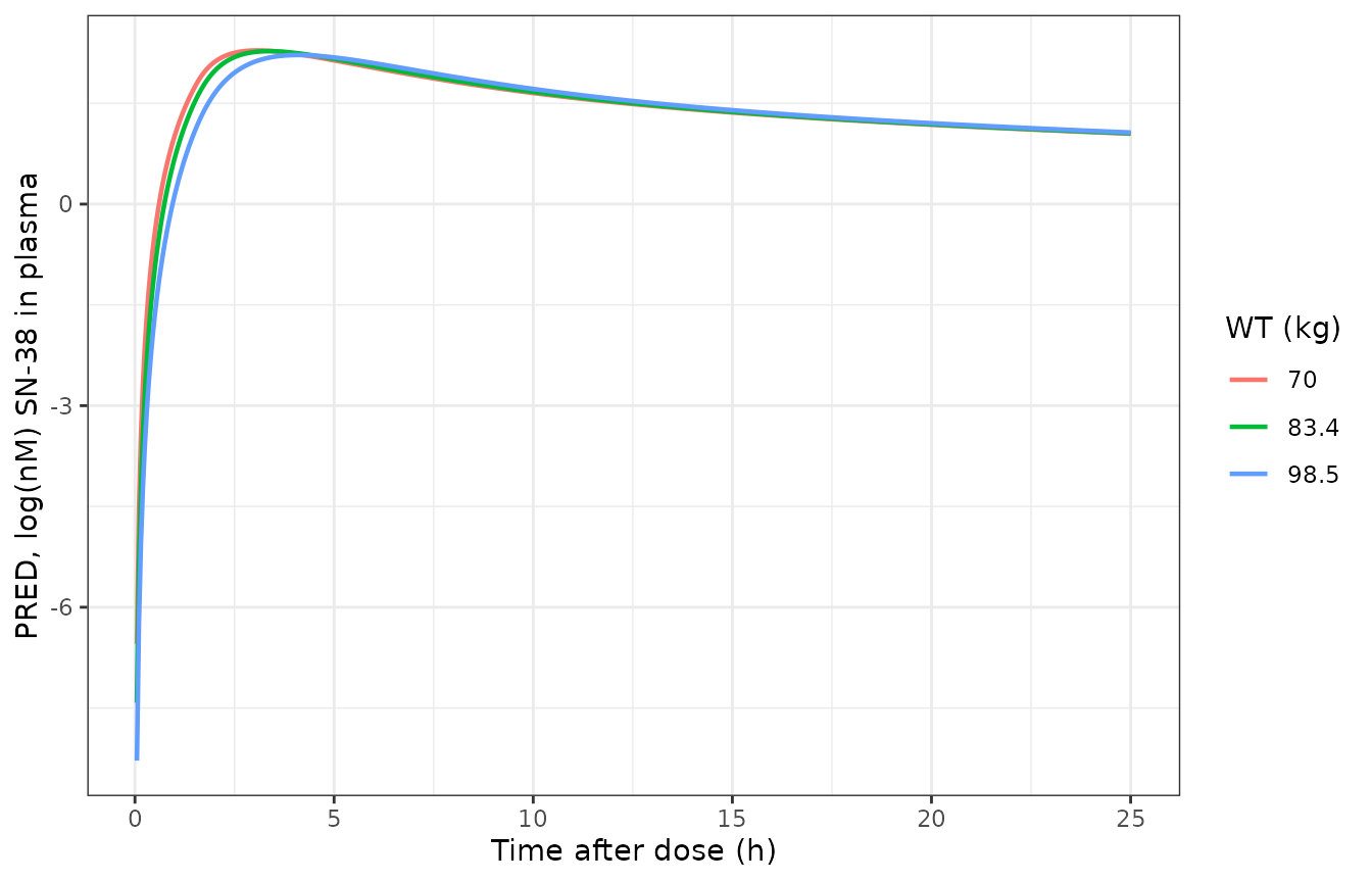
Replicates Figure 2 of Rietveld 2024: effect of weight on SN-38 plasma PRED at the 75 mg dose.
Replicating Figure 3 – GGT on SN-38 plasma clearance
Paper Figure 3 uses the Q1 / median / Q3 GGT values 26 / 32 / 62 U/L. The exponent is negative, so higher GGT lowers SN-38 clearance and raises the concentrations.
ggt_q <- c(26, 32, 62)
fig3 <- solve_typical(dose_umol[["75 mg"]], wt = rep(WT_REF, 3), ggt = ggt_q)
#> ℹ omega/sigma items treated as zero: 'etalcl_sn38', 'etalvc_sn38'
#> Warning: multi-subject simulation without without 'omega'

ggplot(dplyr::filter(fig3, time > 0, time <= 25),
       aes(time, log(Cc_sn38 * 1000), colour = factor(GGT))) +
  geom_line(linewidth = 0.8) +
  labs(x = "Time after dose (h)", y = "PRED, log(nM) SN-38 in plasma",
       colour = "GGT (U/L)") +
  theme_bw()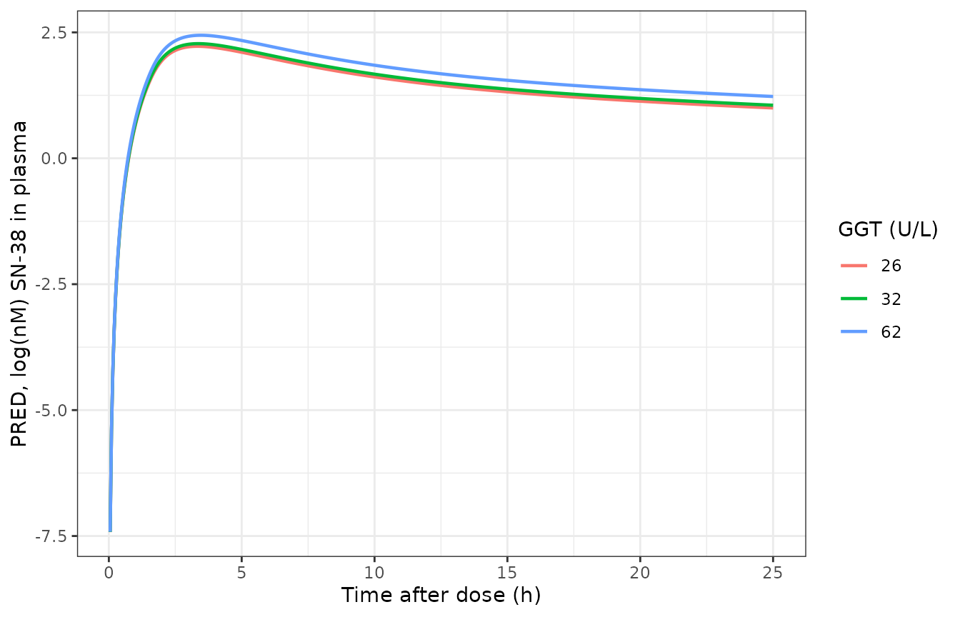
Replicates Figure 3 of Rietveld 2024: effect of GGT on SN-38 plasma PRED at the 75 mg dose.
# Higher GGT must raise SN-38 plasma exposure; the published exponent
# -0.26 fixes the ratio exactly, so this is a closed-form check against
# the printed Equation 3 rather than a shape impression.
auc_by_ggt <- vapply(split(fig3, fig3$GGT), function(d) {
  d <- d[order(d$time), ]
  sum(diff(d$time) * (head(d$Cc_sn38, -1) + tail(d$Cc_sn38, -1)) / 2)
}, numeric(1))
observed_ratio <- auc_by_ggt[["62"]] / auc_by_ggt[["26"]]
expected_ratio <- (62 / 26)^(0.26)   # AUC scales as 1 / CL_M
stopifnot(abs(observed_ratio / expected_ratio - 1) < 0.02)
c(observed = observed_ratio, expected = expected_ratio)
#> observed expected
#> 1.252372 1.253513
Mass-balance gates
These are exact identities implied by paper Figure 1 and the Table 2
values. Both sides are computed independently – the left-hand side from
a numerical solve, the right-hand side in closed form from the printed
parameters – so a transcription error in ka_ip,
kmet_ip, fm, Ka2 or either
clearance makes them disagree.
long <- solve_typical(dose_umol[["75 mg"]], wt = WT_REF, ggt = GGT_REF)
#> ℹ omega/sigma items treated as zero: 'etalcl_sn38', 'etalvc_sn38'
# Extend far past 48 h so the integrals approximate AUC(0, Inf).
ev_long <- make_events(dose_umol[["75 mg"]], ids = 1L, wt = WT_REF,
                       ggt = GGT_REF, obs_times = seq(0, 2000, by = 0.5))
sol <- as.data.frame(rxode2::rxSolve(rxode2::zeroRe(mod), ev_long,
                                     useLinCmt = FALSE))
#> ℹ omega/sigma items treated as zero: 'etalcl_sn38', 'etalvc_sn38'
trapz <- function(y, x) sum(diff(x) * (head(y, -1) + tail(y, -1)) / 2)

auc_iri <- trapz(sol$Cc, sol$time)
auc_sn_p <- trapz(sol$Cc_sn38, sol$time)
auc_sn_ip <- trapz(sol$Cip_sn38, sol$time)

D <- dose_umol[["75 mg"]]
ka <- 1.02; kmet <- 0.118; CL <- 33.2; CLM <- 46; fm <- 0.03; Ka2 <- 4.68

# 1. Fraction of the instilled dose that reaches plasma as irinotecan.
frac_absorbed <- ka / (ka + kmet)
stopifnot(abs(auc_iri * CL / (D * frac_absorbed) - 1) < 0.01)

# 2. Everything converted in the peritoneum eventually reaches SN-38 plasma.
frac_converted <- kmet / (ka + kmet)
stopifnot(abs(Ka2 * auc_sn_ip / (D * frac_converted) - 1) < 0.01)

# 3. SN-38 cleared from plasma equals systemic conversion plus IP absorption.
sn38_in <- fm * CL * auc_iri + Ka2 * auc_sn_ip
stopifnot(abs(CLM * auc_sn_p / sn38_in - 1) < 0.01)

c(frac_absorbed = frac_absorbed, frac_converted = frac_converted)
#>  frac_absorbed frac_converted
#>      0.8963093      0.1036907
Virtual cohort and visual predictive check
A cohort of 100 subjects per dose arm (300 total, within the 200-per-arm cap). Weight is sampled over the 60-100 kg range the authors declare the model valid for; GGT is log-normal around the published median. Only the Q1 / median / Q3 of each covariate are published, so the distribution shapes are an assumption (see Assumptions and deviations).
rxode2::rxSetSeed(20240613)
set.seed(20240613)

n_per_arm <- 100L
cohort <- lapply(seq_along(doses_mg), function(k) {
  ids <- (k - 1L) * n_per_arm + seq_len(n_per_arm)
  wt <- pmin(pmax(rlnorm(n_per_arm, log(WT_REF), 0.16), 60), 100)
  ggt <- pmin(pmax(rlnorm(n_per_arm, log(GGT_REF), 0.65), 10), 200)
  data.frame(id = ids, WT = wt, GGT = ggt,
             treatment = names(dose_umol)[k],
             amt_umol = dose_umol[[k]])
})
cohort <- dplyr::bind_rows(cohort)

events <- dplyr::bind_rows(lapply(split(cohort, cohort$treatment), function(d) {
  ev <- make_events(d$amt_umol[1], ids = d$id, wt = d$WT, ggt = d$GGT,
                    obs_times = sort(unique(c(seq(0, 6, by = 0.25),
                                              seq(6, 48, by = 0.5)))))
  ev$treatment <- d$treatment[1]
  ev
}))

summary(cohort[, c("WT", "GGT")])
#>        WT              GGT
#>  Min.   : 60.00   Min.   : 10.00
#>  1st Qu.: 76.75   1st Qu.: 20.21
#>  Median : 84.88   Median : 30.43
#>  Mean   : 84.76   Mean   : 38.46
#>  3rd Qu.: 94.33   3rd Qu.: 48.74
#>  Max.   :100.00   Max.   :191.73
rxode2::rxSetSeed(20240613)
sim <- as.data.frame(rxode2::rxSolve(
  mod, events,
  keep = c("WT", "GGT", "treatment"),
  useLinCmt = FALSE
))
nrow(sim)
#> [1] 32700
Paper Figure 4 shows a three-panel VPC on the Log(nM)
scale. The panels below reproduce the same three streams from the
model.
vpc <- sim |>
  dplyr::filter(time > 0) |>
  dplyr::select(id, time, treatment, Cc, Cc_sn38, Cip_sn38) |>
  tidyr::pivot_longer(c(Cc, Cc_sn38, Cip_sn38),
                      names_to = "stream", values_to = "conc") |>
  dplyr::mutate(
    stream = factor(stream, levels = c("Cc", "Cc_sn38", "Cip_sn38"),
                    labels = c("IRI central compartment",
                               "SN-38 central compartment",
                               "SN-38 IP compartment")),
    log_nM = log(conc * 1000)
  ) |>
  dplyr::group_by(stream, time) |>
  dplyr::summarise(p10 = quantile(log_nM, 0.10),
                   p50 = median(log_nM),
                   p90 = quantile(log_nM, 0.90),
                   .groups = "drop")

ggplot(vpc, aes(time, p50)) +
  geom_ribbon(aes(ymin = p10, ymax = p90), fill = "steelblue", alpha = 0.30) +
  geom_line(linewidth = 0.7) +
  facet_wrap(~stream) +
  labs(x = "Time after dose (hours)", y = "Log(nM)") +
  theme_bw()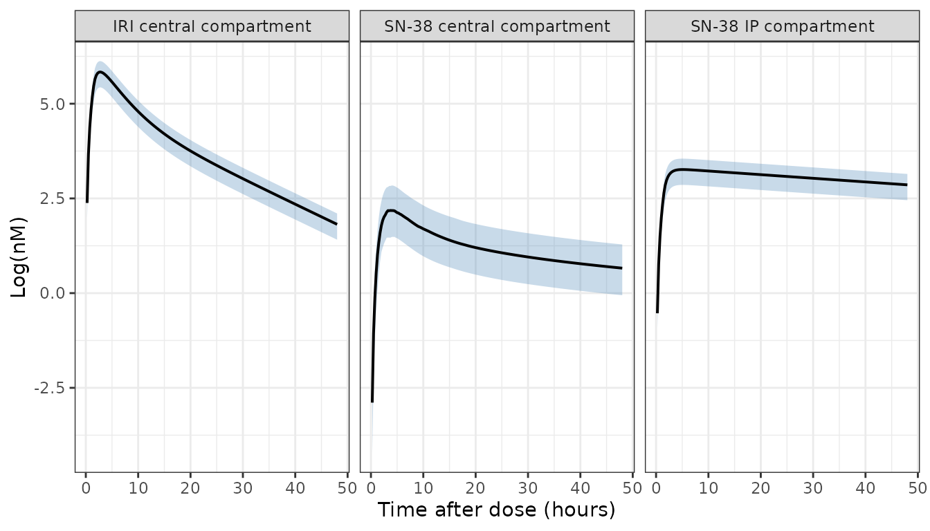
Replicates Figure 4 of Rietveld 2024: median and 10th/90th percentiles for irinotecan in plasma, SN-38 in plasma and SN-38 in peritoneal fluid.
# Anchors digitised from the published Figure 4 panels (median lines).
# Generous windows because they are read off a figure, but tight enough
# that a wrong volume, clearance or unit system falls outside.
peak_log_nM <- sim |>
  dplyr::group_by(id) |>
  dplyr::summarise(iri = log(max(Cc) * 1000),
                   sn_p = log(max(Cc_sn38) * 1000),
                   sn_ip = log(max(Cip_sn38) * 1000),
                   .groups = "drop")

med <- vapply(peak_log_nM[, -1], median, numeric(1))
stopifnot(
  med[["iri"]]   > 5.0 && med[["iri"]]   < 6.5,   # Figure 4 left,   ~5.7-6.0
  med[["sn_p"]]  > 1.7 && med[["sn_p"]]  < 3.0,   # Figure 4 centre, ~2.3
  med[["sn_ip"]] > 2.5 && med[["sn_ip"]] < 3.9    # Figure 4 right,  ~3.0-3.2
)
round(med, 2)
#>   iri  sn_p sn_ip
#>  5.84  2.25  3.26
PKNCA validation
NCA on the simulated irinotecan plasma concentrations, grouped by dose arm, over the 0-24 h interval the paper reports in Table 3.
sim_nca <- sim |>
  dplyr::filter(!is.na(Cc)) |>
  dplyr::select(id, time, Cc, treatment)

# Guarantee a time-zero record (pre-dose Cc = 0 for this extravascular model).
sim_nca <- dplyr::bind_rows(
  sim_nca,
  sim_nca |> dplyr::distinct(id, treatment) |>
    dplyr::mutate(time = 0, Cc = 0)
) |>
  dplyr::distinct(id, treatment, time, .keep_all = TRUE) |>
  dplyr::arrange(id, treatment, time)

dose_df <- cohort |>
  dplyr::transmute(id, time = 0, amt = amt_umol, treatment)

conc_obj <- PKNCA::PKNCAconc(sim_nca, Cc ~ time | treatment + id,
                             concu = "umol/L", timeu = "h")
dose_obj <- PKNCA::PKNCAdose(dose_df, amt ~ time | treatment + id,
                             doseu = "umol")

intervals <- data.frame(start = 0, end = 24,
                        cmax = TRUE, tmax = TRUE, auclast = TRUE)

nca_res <- PKNCA::pk.nca(
  PKNCA::PKNCAdata(conc_obj, dose_obj, intervals = intervals)
)
Comparison against the published NCA
Paper Table 3 reports the geometric-mean irinotecan plasma AUC(0-24 h) per dose group, in ngh/mL; those are converted to umolh/L here so both sides of the table are in the model’s units.
published <- tibble::tribble(
  ~treatment, ~auclast,
  "50 mg",    892.8  / MW_IRI,
  "75 mg",    1947.1 / MW_IRI,
  "100 mg",   2391.7 / MW_IRI
)

cmp <- nlmixr2lib::ncaComparisonTable(
  simulated = nca_res,
  reference = published,
  by = "treatment",
  params = "auclast",
  units = c(auclast = "umol*h/L"),
  tolerance_pct = 20
)

knitr::kable(
  cmp,
  caption = "Simulated vs. published irinotecan plasma AUC(0-24 h). * differs from reference by >20%.",
  align = c("l", "l", "r", "r", "r")
)| NCA parameter | treatment | Reference | Simulated | % diff |
|---|---|---|---|---|
| AUClast (umol*h/L) | 50 mg | 1.52 | 1.99 | +31.1%* |
| AUClast (umol*h/L) | 75 mg | 3.32 | 2.99 | -9.9% |
| AUClast (umol*h/L) | 100 mg | 4.08 | 3.99 | -2.2% |
attr(cmp, "footnote")
#> [1] "* differs from reference by more than ±20%."
pct <- as.numeric(gsub("[^0-9.-]", "", cmp$`% diff`))
names(pct) <- cmp$treatment

# The 75 mg arm is the MTD and the modal dose group (n = 9), so it carries
# the most reliable published geometric mean; the 50 mg (n = 4) and
# 100 mg (n = 5) groups are small and the observed AUCs are not
# dose-proportional (892.8 / 1947.1 / 2391.7 ng*h/mL for a 2-fold dose
# range) while a linear model necessarily is. Assert on the centre, and
# keep only a wide envelope on the small arms.
stopifnot(abs(pct[["75 mg"]]) < 20)
stopifnot(all(abs(pct) < 45))
round(pct, 1)
#>  50 mg  75 mg 100 mg
#>   31.1   -9.9   -2.2
Assumptions and deviations
-
Molar units. Paper Figure 4 plots concentrations as
Log(nM), so the fit was on a molar scale and parent-to-metabolite transfer is equimolar. The model therefore carries no molecular-weight factor. Doses in this vignette are converted from mg using the irinotecan free-base molecular weight 586.68 g/mol; the trial reported doses in mg without stating whether they refer to free base or to the hydrochloride trihydrate salt. A salt-form correction would scale all simulated concentrations by a constant factor of about 0.87. -
Ka2 is a clearance, not a rate constant. Table 2
tabulates
Ka2in L/h even though the abbreviation list calls it “SN-38 absorption”, so the transfer out of the peritoneal SN-38 pool isKa2 / V5. Reading it as a 1/h rate constant instead makes the SN-38 IP concentrations roughly 60-fold too low and contradicts the paper’s own Figure 4. - Weight enters V4, not clearance. The Results sentence introducing Equation 2 says weight acts on “SN-38 plasma clearance”, but the Abstract, the Table 2 footnote (“WT, weight on SN-38 central volume of distribution”), the Figure 2 caption, the covariate-screening sentence and the Discussion all place weight on the SN-38 central volume. The volume reading is used.
- Weight normalisation constant. Equation 2 and the Figure 2 legend both use 83.4 kg as the population median, while Table 1 reports a baseline weight median of 79.7 kg. The printed equation value (83.4 kg) is used. The authors state the model is only applicable over 60-100 kg, and the virtual cohort respects that.
-
Residual error read as a log-scale SD. Table 2
reports the three
Add ERR CMTrows without a scale label. They are taken here as standard deviations on the natural-log scale, i.e. proportional errors in linear space, consistent with the same table reporting the two IIV terms as CV%. If they were instead NONMEM$SIGMAvariances, the corresponding SDs would be 0.653, 0.497 and 0.766. This affects only the width of the simulated prediction intervals, not any typical-value result in this vignette. -
Irinotecan carries no IIV. The Table 2 footnote
defines
IIV-CLandIIV-V2, but neither appears in the table and the Results state that IIV was retained only on SN-38 plasma clearance and the SN-38 central volume. The footnote is treated as a leftover from an earlier model version. Consequently all between-subject variability in the irinotecan stream is absorbed into its residual error. - Covariate distributions are assumed. Only Q1 / median / Q3 are published for weight (70 / 83.4 / 98.5 kg) and GGT (26 / 32 / 62 U/L), and GGT is not tabulated in Table 1 at all. The virtual cohort samples log-normal distributions matched to those medians and truncated to plausible ranges; the published quantiles are used directly for the Figure 2 and Figure 3 replications, which are typical-value curves and do not depend on the assumed distribution.
-
Compartment specimen labels. SN-38 was assayed in
peritoneal fluid (263 samples), but the
compartmentDataspecimen vocabulary inR/conventions.Rhas no “peritoneal fluid” matrix. Both peritoneal states are depot states and carry the vocabulary’s designated depot label “administration site”; the assayed matrix is recorded in the model file comments and here. - Supplement not available. The supplement for PMC11179701 was not available when this model was built. The supplement contains Figures S1-S9 (concentration-time data, goodness-of-fit panels and the ex-vivo carboxylesterase experiments) and no parameter values; every value in the model file comes from the main-text Table 2 and Equations 2-3, so nothing needed for the model is missing.
Errata
The derived SN-38 AUC summary values in the Results do not reproduce from the published model. The paper reports “median (min-max) SN-38 AUCs were 43 (17-85) ng h/mL and 205.4 (136-299) ng h/mL for plasma and peritoneal fluid respectively”, stating that these were “computed using our developed population PK model”. Solving the published model with the published Table 2 parameters at the modal 75 mg dose gives materially larger values.
errata <- tibble::tribble(
  ~Quantity,                            ~`Paper Results text`, ~`This model`,
  "Irinotecan plasma AUC(0-24 h), ng*h/mL", 1947.1,
    round(trapz(long$Cc[long$time <= 24], long$time[long$time <= 24]) * MW_IRI, 1),
  "SN-38 plasma AUC(0-48 h), ng*h/mL",      43.0,
    round(trapz(long$Cc_sn38, long$time) * MW_SN, 1),
  "SN-38 peritoneal AUC(0-48 h), ng*h/mL",  205.4,
    round(trapz(long$Cip_sn38, long$time) * MW_SN, 1)
)
knitr::kable(errata, caption = "Derived AUC values: paper Results text vs. the published model re-solved.")| Quantity | Paper Results text | This model |
|---|---|---|
| Irinotecan plasma AUC(0-24 h), ng*h/mL | 1947.1 | 1755.4 |
| SN-38 plasma AUC(0-48 h), ng*h/mL | 43.0 | 68.9 |
| SN-38 peritoneal AUC(0-48 h), ng*h/mL | 205.4 | 399.6 |
The irinotecan plasma AUC – the only one of the three that the paper also reports from the observed data, in Table 3 – agrees. The two SN-38 values disagree by roughly 1.6-fold and 2-fold.
The paper’s own Figure 4 VPC adjudicates this, and it sides with the
model rather than with the Results text. Reading the median lines off
the three panels gives roughly Log(nM) = 5.7-6.0 for
irinotecan plasma, 2.3 for SN-38 plasma, and a near-flat 3.0-3.2 for
SN-38 peritoneal fluid; the model reproduces all three (see the Figure 4
replication check above). Integrating the peritoneal panel by eye (about
e^3.1 = 22 nM held over 48 h) gives roughly 1.06 umolh/L, close to
the model’s value and about twice the 205.4 ngh/mL (0.52 umol*h/L)
quoted in the text.
The model file therefore reproduces the published model; the
Results-text AUC summaries appear to be inconsistent with it. No
parameter was adjusted to reconcile them. Note also that the authors
themselves flag the peritoneal SN-38 compartment as the weakest part of
the fit: V5 was fixed because it was highly correlated with
CL_PM, and Figure 4 shows the model does not capture the
fast early IP SN-38 formation.
Two further internal inconsistencies, neither of which affects the model:
- The Abstract reports 588 plasma and 267 peritoneal-fluid samples,
while the Results report 334 + 258 = 592 plasma and 263 peritoneal
samples. The Results counts are used in the
populationmetadata. - The Discussion quotes an SN-38 AUC(IP/IV) ratio of 5.8, while the Results give 4.8 (which is what 205.4 / 43 equals).