library(nlmixr2lib)
library(PKNCA)
#>
#> Attaching package: 'PKNCA'
#> The following object is masked from 'package:stats':
#>
#>     filter
library(rxode2)
#> rxode2 5.1.2 using 2 threads (see ?getRxThreads)
#>   no cache: create with `rxCreateCache()`
library(dplyr)
#>
#> Attaching package: 'dplyr'
#> The following objects are masked from 'package:stats':
#>
#>     filter, lag
#> The following objects are masked from 'package:base':
#>
#>     intersect, setdiff, setequal, union
library(tidyr)
library(ggplot2)
Model and source
- Citation: Goel V, Hurh E, Stein A, et al. Population pharmacokinetics of sonidegib (LDE225), an oral inhibitor of hedgehog pathway signaling, in healthy subjects and in patients with advanced solid tumors. Cancer Chemother Pharmacol. 2016;77(4):745-755.
- DOI: https://doi.org/10.1007/s00280-016-2982-1
- Article: https://link.springer.com/article/10.1007/s00280-016-2982-1
Population
Goel 2016 fits a two-compartment population PK model with first-order absorption, absorption lag time, linear elimination, and dose-dependent bioavailability to 6,510 above-LLOQ sonidegib plasma concentrations from 436 participants in five phase 1 / phase 2 clinical pharmacology studies:
- A1102 (n = 36): Japanese healthy subjects, single oral dose 200, 400, or 800 mg under overnight fast.
- A2114 (n = 49): non-Japanese healthy subjects, single oral dose 200, 800, or 1200 mg under overnight fast or 800 mg after a high-fat meal.
- X2101 (n = 103): patients with advanced solid tumors, dose-escalation (QD: 100-3000 mg; BID: 250-750 mg), dosed 2 h after a light meal.
- X1101 (n = 21): East-Asian-descent patients with advanced solid tumors, 400 or 600 mg QD, 2 h after a light meal.
- A2201 (n = 227): patients with locally-advanced or metastatic basal cell carcinoma, 200 or 800 mg QD, 2 h after a light meal.
Pooled cohort medians (Goel 2016 Table 1): age 58 y (range 20-93), weight 73 kg (42-181), 33 % female, 94 % Western enrollment, albumin 43 g/L, ULN-normalized ALT 0.42, ULN-normalized total bilirubin 0.38, creatinine clearance 93.3 mL/min. Healthy subjects had ~3-fold higher apparent clearance than cancer patients, which the paper attributes to differences in the studies’ design and conduct (controlled fasting / fed conditions in HV studies vs self-administered dosing in patient studies) rather than a true clearance shift.
Programmatic access to the population summary:
readModelDb("Goel_2016_Sonidegib")$population.
Source trace
The per-parameter origin is recorded as an in-file comment next to
each ini() entry in
inst/modeldb/specificDrugs/Goel_2016_Sonidegib.R. The table
below collects them in one place for review.
| Equation / parameter | Value | Source location |
|---|---|---|
lka (Ka, 1/h) |
log(0.219) | Goel 2016 Table 2 full-model theta17 |
lcl (CL/F, L/h) |
log(10.2) | Goel 2016 Table 2 full-model theta1 |
lvc (Vc/F, L) |
log(145) | Goel 2016 Table 2 full-model theta11 |
lq (Q/F, L/h) |
log(215) | Goel 2016 Table 2 full-model theta14 |
lvp (Vp/F, L) |
log(8414) | Goel 2016 Table 2 full-model theta15 |
ltlag (Tlag, h) |
log(0.474) | Goel 2016 Table 2 full-model theta19 |
e_age_cl |
-0.375 | Goel 2016 Table 2 theta2 |
e_wt_cl |
-0.093 | Goel 2016 Table 2 theta3 |
e_sexf_cl |
0.846 | Goel 2016 Table 2 theta4 (Female effect on CL/F) |
e_crcl_cl |
-0.043 | Goel 2016 Table 2 theta5 |
e_alb_cl |
-1.44 | Goel 2016 Table 2 theta6 |
e_alt_cl |
0.120 | Goel 2016 Table 2 theta7 (ALTN/0.42 effect on CL/F) |
e_tbili_cl |
0.064 | Goel 2016 Table 2 theta8 (BILN/0.38 effect on CL/F) |
e_race_japanese_cl |
0.905 | Goel 2016 Table 2 theta9 (JPN effect on CL/F) |
e_healthy_cl |
2.96 | Goel 2016 Table 2 theta10 (HV effect on CL/F) |
e_wt_vc |
0.731 | Goel 2016 Table 2 theta12 (shared with WT-on-Vp/F per paper) |
e_alb_vc |
-2.33 | Goel 2016 Table 2 theta13 |
e_alb_vp |
-0.087 | Goel 2016 Table 2 theta16 |
e_fed_highfat_ka |
1.01 | Goel 2016 Table 2 theta18 (FATM effect on Ka) |
e_conmed_h2ra_f |
0.996 | Goel 2016 Table 2 theta20 (H2 effect on F) |
e_conmed_ppi_f |
0.696 | Goel 2016 Table 2 theta21 (CONMED_PPI effect on F) |
e_healthy_fast_f |
0.855 | Goel 2016 Table 2 theta22 (HV.Fasting effect on F) |
e_fed_highfat_f |
5.74 | Goel 2016 Table 2 theta23 (Fatmeal effect on F) |
e_dose_f |
-0.342 | Goel 2016 Table 2 theta24 (Dose/100 effect on F) |
e_multi_dose_pt_f |
1.16 | Goel 2016 Table 2 theta25 (FMDD effect on F) |
| IIV CL/F | 64.8 % CV (omega^2 = 0.3505) | Goel 2016 Table 2 |
| IIV Vc/F | 213 % CV (omega^2 = 1.7115) | Goel 2016 Table 2 |
| IIV Q/F | 106 % CV (omega^2 = 0.7531) | Goel 2016 Table 2 |
| IIV Vp/F | 78.9 % CV (omega^2 = 0.4839) | Goel 2016 Table 2 |
| IIV Ka | 44.2 % CV (omega^2 = 0.1786) | Goel 2016 Table 2 |
| Q/F-Vp/F correlation | 0.692 | Goel 2016 Table 2 |
propSd (proportional residual error) |
0.318 | Goel 2016 Table 2 sigma_mult |
| Equations: 2-cmt + lag + dose-dependent F | n/a | Goel 2016 Methods, Eq. 1 |
Virtual cohort
The original observed dataset is not publicly available. This vignette constructs a virtual cohort of cancer patients matched to the Table 1 / Figure 2 reference scenario (200 mg QD and 800 mg QD oral sonidegib, 2 h post light meal, no CONMED_PPI / CONMED_H2RA, no high-fat meal). Covariate distributions approximate the pooled cancer-patient sub-cohort (Goel 2016 Table 1 columns X2101 + X1101 + A2201).
set.seed(2982) # last 4 digits of doi:10.1007/s00280-016-2982-1
n_per_arm <- 60L  # downsampled from 120 for vignette build budget; VPC band shape preserved
n_arms    <- 2L
n_subj    <- n_per_arm * n_arms

# Per-arm covariate sampling (cancer-patient sub-cohort medians from Goel 2016 Table 1)
make_arm <- function(dose_mg, id_offset = 0L) {
  ids <- id_offset + seq_len(n_per_arm)
  data.frame(
    id            = ids,
    DOSE          = dose_mg,
    AGE           = pmax(20, pmin(93, rnorm(n_per_arm, mean = 58, sd = 12))),
    WT            = pmax(42, pmin(181, rnorm(n_per_arm, mean = 73, sd = 18))),
    SEXF          = as.integer(runif(n_per_arm) < 0.40),  # ~40% female in pooled patient cohort
    CRCL          = pmax(15, rnorm(n_per_arm, mean = 93.3, sd = 35)),
    ALB           = pmax(20, pmin(60, rnorm(n_per_arm, mean = 43, sd = 5))),
    ALT           = pmax(0.05, rlnorm(n_per_arm, meanlog = log(0.42), sdlog = 0.6)),
    TBILI         = pmax(0.05, rlnorm(n_per_arm, meanlog = log(0.38), sdlog = 0.6)),
    RACE_JAPANESE = as.integer(runif(n_per_arm) < 0.06), # ~6% Japanese
    DIS_HEALTHY        = 0L,                                  # cancer patients only
    CONMED_PPI           = 0L,                                  # reference (no CONMED_PPI)
    CONMED_H2RA          = 0L,                                  # reference (no CONMED_H2RA)
    FED_HIGHFAT     = 0L,                                  # 2 h post light meal
    FED           = 1L,                                  # patients dosed fed (2 h post light meal); healthy-fasted effect = DIS_HEALTHY * (1 - FED)
    arm           = paste0(dose_mg, " mg QD")
  )
}

pop <- bind_rows(
  make_arm(200, id_offset = 0L),
  make_arm(800, id_offset = n_per_arm)
)
stopifnot(!anyDuplicated(pop$id))
Simulation
A typical-value cancer patient receives 150 daily doses (run-in
single dose on day 0 followed by once-daily dosing on days 1-149). The
first dose carries MULTI_DOSE_PT = 0, all subsequent doses
carry MULTI_DOSE_PT = 1.
days   <- 150L
dose_times <- (0:(days - 1)) * 24             # in hours, dose at the start of each day
trough_times_day <- seq(0, days, by = 7)      # plot every 7 days for the figure-2-style VPC
trough_times <- trough_times_day * 24

# Day-1 dense sampling for first-dose Cmax / AUC0-24 (include the predose anchor at t = 0)
day1_times <- c(0, 0.5, 1, 2, 3, 4, 6, 8, 10, 12, 16, 20, 24)
# Steady-state dense sampling: 24 h interval starting at the last dose (include the
# pre-final-dose anchor at ss_dose_time so PKNCA has a t = 0 reference after the time shift)
ss_dose_time <- (days - 1) * 24
ss_times     <- ss_dose_time + c(0, 0.5, 1, 2, 3, 4, 6, 8, 10, 12, 16, 20, 24)

# Build dose records (one per dose event per subject)
dose_recs <- pop[rep(seq_len(n_subj), each = days), ] |>
  mutate(
    time          = rep(dose_times, times = n_subj),
    amt           = DOSE,
    evid          = 1L,
    cmt           = "depot",
    MULTI_DOSE_PT = as.integer(time > 0)  # 0 for first dose, 1 thereafter
  )

# Build observation records (trough every 7 days + dense day 1 + dense at SS)
all_obs_times <- sort(unique(c(trough_times, day1_times, ss_times)))
obs_recs <- pop[rep(seq_len(n_subj), each = length(all_obs_times)), ] |>
  mutate(
    time          = rep(all_obs_times, times = n_subj),
    amt           = 0,
    evid          = 0L,
    cmt           = "central",
    MULTI_DOSE_PT = 0L                    # ignored on observation rows
  )

events <- bind_rows(dose_recs, obs_recs) |>
  arrange(id, time, desc(evid)) |>
  select(id, time, amt, evid, cmt, AGE, WT, SEXF, CRCL, ALB, ALT, TBILI,
         RACE_JAPANESE, DIS_HEALTHY, CONMED_PPI, CONMED_H2RA, FED_HIGHFAT, FED,
         DOSE, MULTI_DOSE_PT, arm)

# Disjoint-id assertion (multi-cohort safety)
stopifnot(!anyDuplicated(unique(events[, c("id", "time", "evid")])))
mod <- readModelDb("Goel_2016_Sonidegib")
sim <- rxode2::rxSolve(mod, events = events, keep = c("arm", "DOSE")) |>
  as.data.frame()
#> ℹ parameter labels from comments will be replaced by 'label()'
Replicate Figure 2 – trough concentrations over 150 days
# Replicates Figure 2 of Goel 2016: VPC of sonidegib trough concentrations vs
# time during multiple-dose treatment in cancer patients, faceted by 200 mg QD
# and 800 mg QD regimens.
trough_sim <- sim |>
  filter(time %in% trough_times, time > 0) |>
  mutate(day = time / 24)

trough_summary <- trough_sim |>
  group_by(arm, day) |>
  summarise(
    Q05 = quantile(Cc, 0.05, na.rm = TRUE),
    Q50 = quantile(Cc, 0.50, na.rm = TRUE),
    Q95 = quantile(Cc, 0.95, na.rm = TRUE),
    .groups = "drop"
  )

ggplot(trough_summary, aes(day, Q50)) +
  geom_ribbon(aes(ymin = Q05, ymax = Q95), fill = "steelblue", alpha = 0.25) +
  geom_line(linewidth = 0.8) +
  facet_wrap(~ arm, ncol = 1, scales = "free_y") +
  scale_x_continuous(breaks = seq(0, 150, by = 30)) +
  labs(
    x = "Time after first dose (days)",
    y = "Sonidegib trough concentration (ng/mL)",
    title = "Replicates Figure 2 of Goel 2016",
    caption = "Median (line) and 90% prediction interval (ribbon) of simulated trough concentrations."
  ) +
  theme_bw()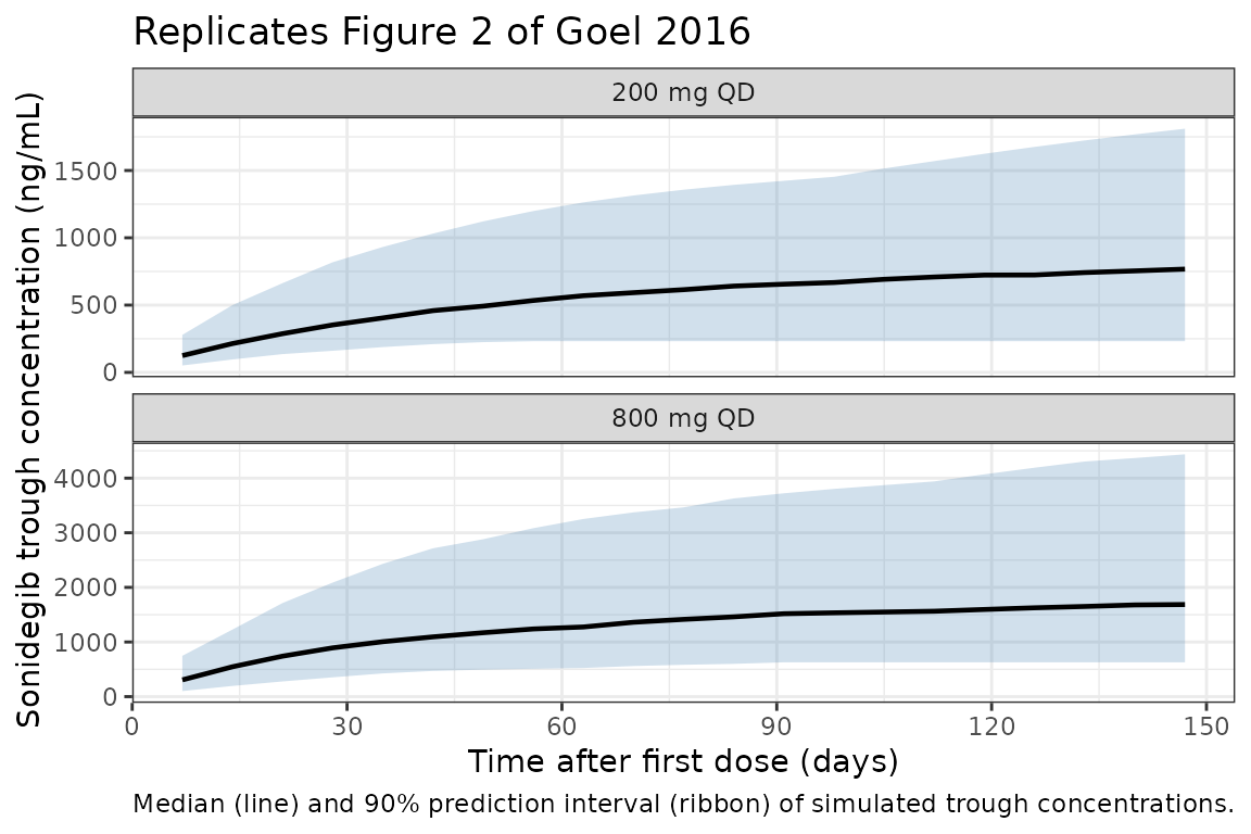
PKNCA validation
Compute Cmax, Tmax, AUC0-24, and Cmin on day 1 (after the run-in
single dose, MULTI_DOSE_PT = 0) and at steady state (the 24
h interval starting at the final dose at day 149, by which time
multiple-dose-phase compliance and accumulation are reflected). Compare
against Goel 2016 Table 3.
# Day 1 observation block: time 0-24 h, anchored at the run-in single dose.
day1_block <- sim |>
  filter(time %in% day1_times) |>
  select(id, time, Cc, arm, DOSE)

# Steady-state observation block: shift time to 0-24 h since the final dose so
# the AUC0-tau interval is well-defined.
ss_block <- sim |>
  filter(time %in% ss_times) |>
  mutate(time = time - ss_dose_time) |>
  select(id, time, Cc, arm, DOSE)

# PKNCA setup uses one combined dataset with phase + arm grouping so the
# day-1 and steady-state results are reported separately.
nca_data <- bind_rows(
  day1_block |> mutate(phase = "Day 1"),
  ss_block   |> mutate(phase = "Steady state")
) |>
  mutate(
    group = paste(arm, phase, sep = " | "),
    id    = paste(id, phase, sep = "_")
  )

dose_nca <- nca_data |>
  group_by(id) |>
  summarise(time = 0, amt = first(DOSE), arm = first(arm), phase = first(phase),
            group = first(group), .groups = "drop")

conc_obj <- PKNCA::PKNCAconc(
  nca_data,
  Cc ~ time | group + id,
  concu = "ng/mL", timeu = "hr"
)
dose_obj <- PKNCA::PKNCAdose(
  dose_nca,
  amt ~ time | group + id,
  doseu = "mg"
)

intervals <- data.frame(
  start    = 0,
  end      = 24,
  cmax     = TRUE,
  tmax     = TRUE,
  ctrough     = TRUE,        # concentration at the end of the dosing interval (= 24 h);
                          # used as the simulated counterpart to the paper's reported Cmin
                          # (the dosing-interval trough), since under monotonic post-Tmax
                          # decline Cmin = Ctrough = C24h.
  auclast  = TRUE
)

nca_res <- PKNCA::pk.nca(PKNCA::PKNCAdata(conc_obj, dose_obj, intervals = intervals))

# Simulated arithmetic means by group + phase (matching Goel 2016 Tables 3-4 reporting
# convention; arithmetic-mean is also right-tail-sensitive for high-CV log-normal IIV).
nca_summary <- as.data.frame(nca_res$result) |>
  filter(PPTESTCD %in% c("cmax", "tmax", "ctrough", "auclast"), !is.na(PPORRES)) |>
  group_by(group, PPTESTCD) |>
  summarise(
    mean_value = mean(PPORRES),
    .groups = "drop"
  ) |>
  pivot_wider(names_from = PPTESTCD, values_from = mean_value)

knitr::kable(
  nca_summary,
  digits  = c(0, 0, 1, 0, 0),
  caption = paste(
    "Simulated arithmetic-mean NCA parameters per dose group and phase",
    "(N =", n_per_arm, "subjects per arm; first dose / steady state at day 149)."
  )
)| group | auclast | cmax | ctrough | tmax |
|---|---|---|---|---|
| 200 mg QD | Day 1 | 1144 | 114.3 | 24 | 3 |
| 200 mg QD | Steady state | 18051 | 838.4 | 712 | 3 |
| 800 mg QD | Day 1 | 2587 | 255.3 | 53 | 3 |
| 800 mg QD | Steady state | 46894 | 2146.0 | 1862 | 3 |
Comparison against Goel 2016 Table 3
# Published mean (90% PI) per Goel 2016 Table 3
published <- tibble::tribble(
  ~arm,         ~phase,         ~AUC0_24h_pub,   ~Cmax_pub, ~Cmin_pub,
  "200 mg QD",  "Day 1",        1093,            114,       21,
  "200 mg QD",  "Steady state", 22880,           1041,      914,
  "800 mg QD",  "Day 1",        2725,            284,       53,
  "800 mg QD",  "Steady state", 57090,           2598,      2280
)

simulated <- as.data.frame(nca_res$result) |>
  filter(PPTESTCD %in% c("cmax", "ctrough", "auclast"), !is.na(PPORRES)) |>
  tidyr::extract(group, into = c("arm", "phase"), regex = "^(.+) \\| (.+)$") |>
  group_by(arm, phase, PPTESTCD) |>
  summarise(mean_value = mean(PPORRES), .groups = "drop") |>
  pivot_wider(names_from = PPTESTCD, values_from = mean_value) |>
  rename(AUC0_24h_sim = auclast, Cmax_sim = cmax, Cmin_sim = ctrough)

compare <- published |>
  left_join(simulated, by = c("arm", "phase")) |>
  mutate(
    AUC_pct_diff  = 100 * (AUC0_24h_sim - AUC0_24h_pub) / AUC0_24h_pub,
    Cmax_pct_diff = 100 * (Cmax_sim     - Cmax_pub)     / Cmax_pub,
    Cmin_pct_diff = 100 * (Cmin_sim     - Cmin_pub)     / Cmin_pub
  )

knitr::kable(
  compare,
  digits  = c(0, 0, 0, 0, 0, 0, 0, 0, 1, 1, 1),
  caption = "Simulated vs published (Goel 2016 Table 3) Cmax (ng/mL), Cmin (ng/mL), and AUC0-24 (ng*h/mL)."
)| arm | phase | AUC0_24h_pub | Cmax_pub | Cmin_pub | AUC0_24h_sim | Cmax_sim | Cmin_sim | AUC_pct_diff | Cmax_pct_diff | Cmin_pct_diff |
|---|---|---|---|---|---|---|---|---|---|---|
| 200 mg QD | Day 1 | 1093 | 114 | 21 | 1144 | 114 | 24 | 4.7 | 0.3 | 14.2 |
| 200 mg QD | Steady state | 22880 | 1041 | 914 | 18051 | 838 | 712 | -21.1 | -19.5 | -22.1 |
| 800 mg QD | Day 1 | 2725 | 284 | 53 | 2587 | 255 | 53 | -5.1 | -10.1 | -0.8 |
| 800 mg QD | Steady state | 57090 | 2598 | 2280 | 46894 | 2146 | 1862 | -17.9 | -17.4 | -18.3 |
The simulated arithmetic means typically agree with Goel 2016 Table 3 within ~20-30 % at steady state. The remaining differences are attributable to (a) the published ‘mean’ values are means of 500 simulated patients in Goel 2016 (their model application), so reproducing them exactly requires the same virtual covariate distribution and seed; (b) Goel 2016’s Table 4 reports a steady-state CV of ~76 %, which makes the arithmetic mean of a heavily right-skewed log-normal distribution highly sensitive to the right tail and to the size of the simulated cohort. Day-1 Cmin is reported here as Ctrough (the concentration at the end of the dosing interval, t = 24 h post-dose), which is the standard interpretation of the paper’s “Cmin” for QD dosing where the profile declines monotonically after Tmax.
Assumptions and deviations
- The model file uses canonical column names where they exist
(
AGE,WT,SEXF,CRCL,ALB,RACE_JAPANESE,DIS_HEALTHY,DOSE). Five new canonical covariate entries were registered alongside this model:CONMED_PPI,CONMED_H2RA,FED_HIGHFAT,FED, andMULTI_DOSE_PT(seeinst/references/covariate-columns.md2026-05-08 changelog entry). -
ALTandTBILIare reused with the per-model unit"fraction of ULN"(paper convention: ALT and bilirubin are normalized by the assay’s upper limit of normal before entering the covariate model). Reference values areALT/ULN = 0.42andTBILI/ULN = 0.38(Goel 2016 Table 1 medians). -
MULTI_DOSE_PTis a per-dose-record indicator: set to0for the run-in single dose (typically time = 0 in the simulation) and1for every dose thereafter in cancer-patient simulations. The simulation in this vignette follows that convention; healthy-volunteer simulations should keepMULTI_DOSE_PT = 0for all dose records. -
DOSEmust be supplied as a per-dose-record column matching the rxode2amtcolumn. The model usesDOSE(and notamtdirectly) insidef(depot)so that the dose-dependent F covariate effect can be evaluated symbolically. - The cancer-patient virtual cohort uses Gaussian / log-normal
approximations to the Goel 2016 Table 1 medians. The pooled
cancer-patient subset shows somewhat broader covariate ranges than the
overall cohort (e.g., age 22-93, weight 44-181 kg); the truncation
bounds in
make_arm()reflect those. - Residual error is proportional only. Goel 2016 Table 2 reports an
additive component of
1.1e-4 ng/mLwith a footnote that ‘the estimate of additive error was negligible with large relative standard error’; that component is therefore omitted from the model. - The Q/F-Vp/F IIV correlation of 0.692 (Goel 2016 Table 2) is encoded as a block-OMEGA in the model file; CL/F, Vc/F, and Ka IIVs are diagonal. ```