Pipamperone (Kloosterboer 2020) • nlmixr2lib

Model and source

Citation: Kloosterboer SM, Egberts KM, de Winter BCM, van Gelder T, Gerlach M, Hillegers MHJ, Dieleman GC, Bahmany S, Reichart CG, van Daalen E, Kouijzer MEJ, Dierckx B, Koch BCP (2020). Pipamperone population pharmacokinetics related to effectiveness and side effects in children and adolescents. Clin Pharmacokinet 59(11):1393-1405. doi:10.1007/s40262-020-00894-y
Description: One-compartment population pharmacokinetic model for oral pipamperone in children and adolescents (5.6-17.7 years) with behavioural problems, pooled from a Dutch prospective observational trial and a German therapeutic-drug-monitoring service (Kloosterboer 2020). First-order absorption with ka fixed at 2 /h; apparent clearance and apparent volume scale allometrically with body weight at fixed exponents 0.75 and 1 referenced to 70 kg. Inter-patient variability on CL/F only. Combined additive + proportional residual error with an extra additive error for samples quantified by HPLC-UV, and a linear conversion of the plasma prediction onto the dried-blood-spot scale for DBS samples.
Article: https://doi.org/10.1007/s40262-020-00894-y
PubMed Central: https://www.ncbi.nlm.nih.gov/pmc/articles/PMC7658071/
Electronic Supplementary Material (external-validation goodness-of-fit and NPDE plots only; no control stream): https://static-content.springer.com/esm/art%3A10.1007%2Fs40262-020-00894-y/MediaObjects/40262_2020_894_MOESM1_ESM.pdf

Population

Kloosterboer 2020 built the model from 70 pipamperone concentrations in 30 children and adolescents: 8 patients from a Dutch multicentre observational trial in autism spectrum disorder with comorbid behavioural problems (SPACe, NTR6050; six samples per patient at random times on two days, by venepuncture and dried blood spot, analysed by UHPLC-MS) and 22 patients from the therapeutic-drug-monitoring service of the University Hospital Wuerzburg (morning trough samples at steady state, analysed by HPLC-UV). Table 1 gives the model-building group as 70% male, median age 13.0 years (range 5.6-17.7), median body weight 50.4 kg (24.8-100.4), median BMI 20.4 kg/m^2, and a median daily dose of 45 mg (12-400 mg) as tablets or oral solution given once to five times daily. Diagnoses were autism spectrum disorder (73.3%), ADHD (40%), mental retardation (30%), schizophrenia-spectrum disorders (6.7%) and conduct disorder (3.3%); 60% took another antipsychotic concomitantly. A further 21 German TDM patients (33 concentrations) were used only for external validation.

The same information is available programmatically:

str(rxode2::rxode(readModelDb("Kloosterboer_2020_pipamperone"))$population)
#> ℹ parameter labels from comments will be replaced by 'label()'
#> List of 11
#>  $ species       : chr "human"
#>  $ n_subjects    : num 30
#>  $ n_studies     : num 2
#>  $ n_observations: num 70
#>  $ age_range     : chr "5.6-17.7 years (median 13.0)"
#>  $ weight_range  : chr "24.8-100.4 kg (median 50.4)"
#>  $ sex_female_pct: num 30
#>  $ disease_state : chr "Children and adolescents treated with pipamperone for behavioural problems: autism spectrum disorder 73.3%, ADH"| __truncated__
#>  $ dose_range    : chr "Oral tablet or oral solution, 12-400 mg/day (median 45 mg/day), once to five times daily"
#>  $ regions       : chr "Netherlands (SPACe trial, n = 8) and Germany (Wuerzburg TDM service, n = 22)"
#>  $ notes         : chr "Model-building group of Kloosterboer 2020 Table 1. An external validation group of 21 German TDM patients (33 c"| __truncated__

Source trace

Model element	Value	Source location
Structure: one compartment, first-order absorption, no lag	–	Section 3.1.1 ‘best described using a one-compartment model’; Section 2.4.1
`lka` (ka)	2 /h, fixed	Table 2 ‘Ka’ = 2, footnote a ‘Fixed’; Section 2.4.1 ‘fixed at 2/h’
`lcl` (CL/F)	22.1 L/h per 70 kg	Table 2 ‘CL/F (L/h/70 kg)’
`lvc` (V/F)	416 L per 70 kg	Table 2 ‘V/F (L/70 kg)’
`e_wt_cl`	0.75, fixed	Table 2 footnote b; Section 3.1.2 ‘fixed exponents’
`e_wt_vc`	1, fixed	Table 2 footnote b
`etalcl`	0.041153 (20.5% CV)	Table 2 ‘IPV CL’ = 20.5%; `log(1 + 0.205^2)`
`addSd`	0.21 ug/L	Table 2 ‘Additional error’
`propSd`	0.39	Table 2 ‘Proportional error’
`addSd_hplc`	26.6 ug/L	Table 2 ‘Additional error HPLC-UV’; Section 3.1.3
`cal_slope_dbs`	0.33	Table 2 ‘DBS correction: y = ax + b’, a
`cal_int_dbs`	3.90 ug/L	Table 2 ‘DBS correction: y = ax + b’, b
Allometric scaling `(WT/70)^0.75` on CL, `(WT/70)^1` on V	–	Section 2.4.1; Table 2 footnote b
DBS prediction `a * Cplasma + b`	–	Table 2 (see Assumptions for the Discussion’s form)
HPLC-UV extra additive error	–	Section 3.1.1 ‘combined error model with an extra additional error for HPLC-UV concentrations’

Typical-value replication of Figure 4

Section 3.3 prints the population-predicted steady-state trough of a twice-daily regimen for a 25, 50 and 75 kg patient, once for a fixed 30 mg dose (Figure 4a) and once for 0.6 mg/kg (Figure 4b: 15, 30 and 45 mg). These are typical values, so they are reproduced exactly with the random effects zeroed.

mod <- readModelDb("Kloosterboer_2020_pipamperone")

regimens <- tibble::tribble(
  ~treatment,           ~WT, ~dose, ~ctrough_pub,
  "30 mg BID, 25 kg",    25,    30,  163.2,
  "30 mg BID, 50 kg",    50,    30,  103.9,
  "30 mg BID, 75 kg",    75,    30,   79.3,
  "0.6 mg/kg BID, 25 kg", 25,   15,   81.6,
  "0.6 mg/kg BID, 50 kg", 50,   30,  103.9,
  "0.6 mg/kg BID, 75 kg", 75,   45,  119.0
) |>
  dplyr::mutate(id = dplyr::row_number())

obs_times <- sort(unique(c(seq(0, 12, by = 0.1), 12)))

make_events <- function(reg) {
  dose_rows <- reg |>
    dplyr::transmute(
      id, treatment, WT,
      time = 0, amt = dose, evid = 1, cmt = "depot", ss = 1, ii = 12
    )
  obs_rows <- reg |>
    dplyr::select(id, treatment, WT) |>
    tidyr::crossing(time = obs_times) |>
    dplyr::mutate(amt = 0, evid = 0, cmt = "central", ss = 0, ii = 0)
  dplyr::bind_rows(dose_rows, obs_rows) |>
    dplyr::mutate(ASSAY_LCMSMS = 1, SAMPLE_DBS = 0) |>
    dplyr::arrange(id, time, dplyr::desc(evid)) |>
    as.data.frame()
}

ev_typ <- make_events(regimens)
sim_typ <- rxode2::rxSolve(rxode2::zeroRe(mod), events = ev_typ,
                           keep = c("treatment", "WT")) |>
  as.data.frame()
#> ℹ parameter labels from comments will be replaced by 'label()'
#> ℹ omega/sigma items treated as zero: 'etalcl'
#> Warning: multi-subject simulation without without 'omega'

sim_typ |>
  dplyr::mutate(
    panel = ifelse(grepl("^30 mg", treatment), "(a) 30 mg BID", "(b) 0.6 mg/kg BID"),
    weight = paste(WT, "kg")
  ) |>
  ggplot(aes(time, Cc, colour = weight)) +
  geom_line(linewidth = 0.8) +
  facet_wrap(~panel) +
  labs(x = "Time after dose (h)", y = "Pipamperone (ug/L)", colour = "Body weight") +
  theme_bw()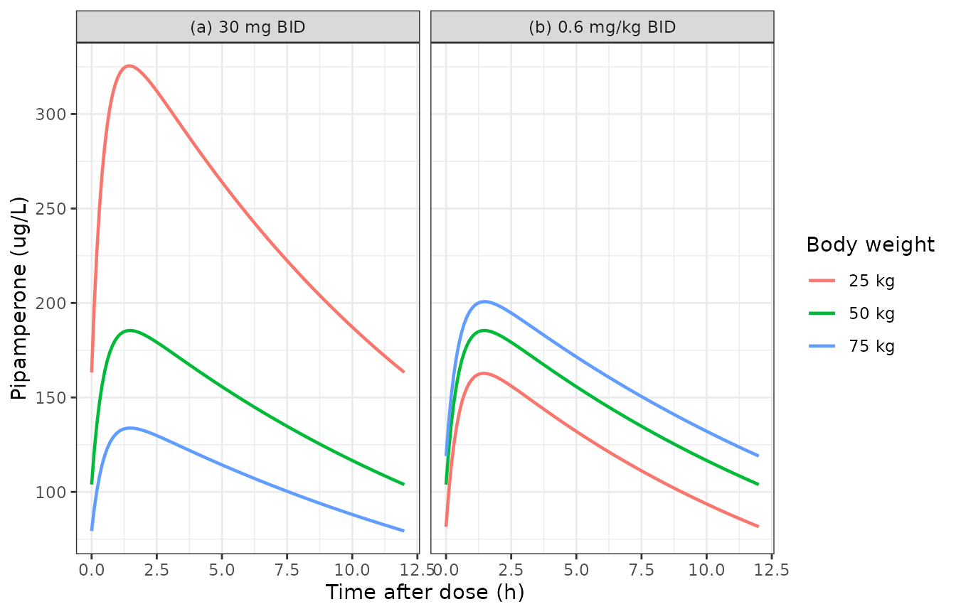

Replicates the population-prediction curves of Figure 4 of Kloosterboer 2020: steady-state twice-daily pipamperone, (a) fixed 30 mg, (b) 0.6 mg/kg.

The trough is also available in closed form for a one-compartment model with first-order absorption at steady state, which checks the ODE solution independently of rxode2:

ss_trough <- function(wt, dose, tau = 12) {
  cl <- 22.1 * (wt / 70)^0.75
  v <- 416 * (wt / 70)
  ka <- 2
  k <- cl / v
  1000 * dose * ka / (v * (ka - k)) *
    (exp(-k * tau) / (1 - exp(-k * tau)) - exp(-ka * tau) / (1 - exp(-ka * tau)))
}

trough_chk <- sim_typ |>
  dplyr::filter(time == 12) |>
  dplyr::select(id, treatment, Cc) |>
  dplyr::left_join(regimens, by = c("id", "treatment")) |>
  dplyr::mutate(
    closed_form = ss_trough(WT, dose),
    pct_vs_paper = 100 * (Cc - ctrough_pub) / ctrough_pub
  )

trough_chk |>
  dplyr::select(treatment, Cc, closed_form, ctrough_pub, pct_vs_paper) |>
  dplyr::rename(
    "Regimen" = treatment,
    "rxode2 trough (ug/L)" = Cc,
    "Closed-form trough (ug/L)" = closed_form,
    "Kloosterboer 2020 Section 3.3 (ug/L)" = ctrough_pub,
    "% difference vs paper" = pct_vs_paper
  ) |>
  knitr::kable(digits = 2)

Regimen	rxode2 trough (ug/L)	Closed-form trough (ug/L)	Kloosterboer 2020 Section 3.3 (ug/L)	% difference vs paper
30 mg BID, 25 kg	163.23	163.23	163.2	0.02
30 mg BID, 50 kg	103.90	103.90	103.9	0.00
30 mg BID, 75 kg	79.33	79.33	79.3	0.03
0.6 mg/kg BID, 25 kg	81.61	81.61	81.6	0.02
0.6 mg/kg BID, 50 kg	103.90	103.90	103.9	0.00
0.6 mg/kg BID, 75 kg	118.99	118.99	119.0	-0.01


stopifnot(
  # Same drawn (typical) parameters on both sides: pure numerical error.
  all(abs(trough_chk$Cc - trough_chk$closed_form) / trough_chk$closed_form < 1e-3),
  # The paper prints the troughs to one decimal place.
  all(abs(trough_chk$pct_vs_paper) < 0.1)
)

All six published troughs are reproduced to the printed precision, which confirms CL/F, V/F, the fixed ka, the 70 kg reference and both allometric exponents together. The typical half-life at 70 kg is 13 h, matching the “mean elimination half-life (13 h)” of the Discussion.

PKNCA on the typical-value profiles

conc_df <- sim_typ |>
  dplyr::filter(!is.na(Cc)) |>
  dplyr::select(id, time, Cc, treatment)

dose_df <- ev_typ |>
  dplyr::filter(evid == 1) |>
  dplyr::select(id, time, amt, treatment)

conc_obj <- PKNCA::PKNCAconc(conc_df, Cc ~ time | treatment + id,
                             concu = "ug/L", timeu = "h")
dose_obj <- PKNCA::PKNCAdose(dose_df, amt ~ time | treatment + id,
                             doseu = "mg")
intervals <- data.frame(start = 0, end = 12, cmax = TRUE, tmax = TRUE,
                        auclast = TRUE, ctrough = TRUE)
nca_res <- PKNCA::pk.nca(PKNCA::PKNCAdata(conc_obj, dose_obj,
                                          intervals = intervals))

simulated_long <- as.data.frame(nca_res$result) |>
  dplyr::select(id, treatment, PPTESTCD, PPORRES)

published <- regimens |>
  dplyr::select(treatment, ctrough = ctrough_pub)

nlmixr2lib::ncaComparisonTable(
  simulated = simulated_long,
  reference = published,
  by = "treatment",
  units = c(cmax = "ug/L", auclast = "ug*h/L", ctrough = "ug/L", tmax = "h"),
  tolerance_pct = 20
) |>
  dplyr::rename("Regimen" = treatment) |>
  knitr::kable(caption = "Typical-value steady-state NCA over one 12 h interval versus the Section 3.3 population-predicted troughs.")

Typical-value steady-state NCA over one 12 h interval versus the Section 3.3 population-predicted troughs.
NCA parameter	Regimen	Reference	Simulated	% diff
Ctrough (ug/L)	30 mg BID, 25 kg	163	163	+0.0%
Ctrough (ug/L)	30 mg BID, 50 kg	104	104	+0.0%
Ctrough (ug/L)	30 mg BID, 75 kg	79.3	79.3	+0.0%
Ctrough (ug/L)	0.6 mg/kg BID, 25 kg	81.6	81.6	+0.0%
Ctrough (ug/L)	0.6 mg/kg BID, 50 kg	104	104	+0.0%
Ctrough (ug/L)	0.6 mg/kg BID, 75 kg	119	119	-0.0%

Kloosterboer 2020 reports only the troughs for these regimens; Cmax, Tmax and AUC are shown for completeness. The 70 kg steady-state AUC over 24 h for a 60 mg daily dose is 2715 ugh/L, in the range of the median predicted AUC24h of the responders (3448 ugh/L) and non-responders (1811 ug*h/L) reported in Section 3.2.1 for the observed doses.

Between-patient variability around the Figure 4 curves

Figure 4 shades a 95% interval from 1000 simulations around each curve. The sketch below simulates 200 virtual patients per weight on the 0.6 mg/kg regimen with between-patient variability on CL/F only; the residual error is not added, so these are individual predictions.

rxode2::rxSetSeed(20200511)
n_per <- 200
reg_iiv <- regimens |>
  dplyr::filter(grepl("^0.6", treatment)) |>
  dplyr::select(treatment, WT, dose) |>
  tidyr::uncount(n_per) |>
  dplyr::mutate(id = dplyr::row_number(), ctrough_pub = NA_real_)

sim_iiv <- rxode2::rxSolve(mod, events = make_events(reg_iiv),
                           keep = c("treatment", "WT")) |>
  as.data.frame()
#> ℹ parameter labels from comments will be replaced by 'label()'

sim_iiv |>
  dplyr::group_by(treatment, time) |>
  dplyr::summarise(
    q025 = quantile(Cc, 0.025), q50 = median(Cc), q975 = quantile(Cc, 0.975),
    .groups = "drop"
  ) |>
  ggplot(aes(time, q50)) +
  geom_ribbon(aes(ymin = q025, ymax = q975), alpha = 0.25) +
  geom_line() +
  facet_wrap(~treatment) +
  labs(x = "Time after dose (h)", y = "Pipamperone (ug/L)") +
  theme_bw()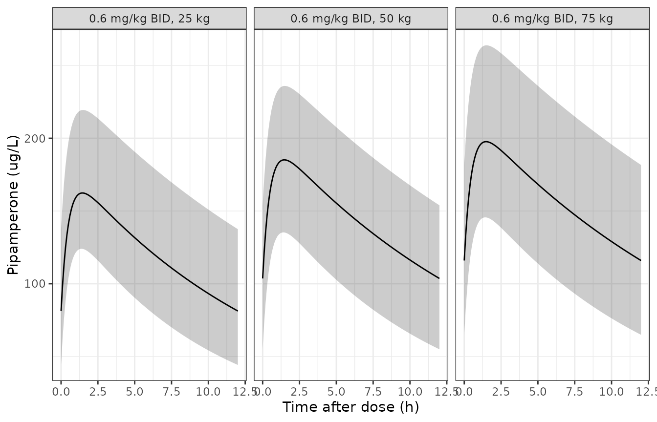


iiv_trough <- sim_iiv |>
  dplyr::filter(time == 12) |>
  dplyr::group_by(treatment) |>
  dplyr::summarise(
    median = median(Cc), p2.5 = quantile(Cc, 0.025), p97.5 = quantile(Cc, 0.975),
    .groups = "drop"
  )
knitr::kable(iiv_trough, digits = 1)

treatment	median	p2.5	p97.5
0.6 mg/kg BID, 25 kg	81.3	44.2	137.5
0.6 mg/kg BID, 50 kg	103.6	54.9	153.9
0.6 mg/kg BID, 75 kg	116.0	64.9	181.6


typ_06 <- trough_chk |> dplyr::filter(grepl("^0.6", treatment))
chk <- dplyr::left_join(iiv_trough, typ_06, by = "treatment")
stopifnot(
  # Centre only: the median of a 200-patient cohort sits near the typical value.
  all(abs(chk$median - chk$Cc) / chk$Cc < 0.1)
)

The published intervals for 0.6 mg/kg (33.6-134.5, 49.0-167.2 and 57.6-186.7 ug/L at 25, 50 and 75 kg) are of similar width to, but somewhat wider and lower-reaching than, the between-patient spread of CL/F alone produces here. The paper does not state which variability components entered its 1000 simulations (residual error at 39% proportional would widen them far more than observed; parameter uncertainty would widen them modestly), so the intervals are shown for orientation and are not used as a gate.

Dried-blood-spot and HPLC-UV observations

A DBS observation row (SAMPLE_DBS = 1) returns the prediction on the DBS scale, 0.33 * Cplasma + 3.90 ug/L. ASSAY_LCMSMS = 0 (HPLC-UV) changes only the residual error.

ev_dbs <- regimens |>
  dplyr::filter(treatment == "0.6 mg/kg BID, 50 kg") |>
  make_events() |>
  dplyr::filter(evid == 1 | time %in% c(2, 12))
ev_dbs2 <- ev_dbs |> dplyr::mutate(SAMPLE_DBS = ifelse(evid == 0, 1, 0))
cc_plasma <- rxode2::rxSolve(rxode2::zeroRe(mod), events = ev_dbs)$Cc
#> ℹ parameter labels from comments will be replaced by 'label()'
#> ℹ omega/sigma items treated as zero: 'etalcl'
cc_dbs <- rxode2::rxSolve(rxode2::zeroRe(mod), events = ev_dbs2)$Cc
#> ℹ parameter labels from comments will be replaced by 'label()'
#> ℹ omega/sigma items treated as zero: 'etalcl'
data.frame(time = c(2, 12), plasma = cc_plasma, dbs = cc_dbs) |>
  knitr::kable(digits = 2)

time	plasma	dbs
2	183.28	64.38
12	103.90	38.19

stopifnot(all(abs(cc_dbs - (0.33 * cc_plasma + 3.90)) < 1e-6))

Assumptions and deviations

DBS conversion direction. Table 2 prints the DBS correction as y = ax + b with a = 0.33 and b = 3.90 ug/L. The model reads this in the natural NONMEM form, DBS prediction = a * plasma prediction + b, which is the only reading of the table’s equation that is consistent with the recovery of pipamperone in DBS being well below 100% (the earlier clinical validation divided DBS values by 0.158). The Discussion instead writes the conversion to plasma as DBS/0.33 + 3.90, which is equivalent to DBS = 0.33 * (plasma - 3.90). The two readings share the slope and differ only in the intercept on the DBS scale (+3.90 versus -1.29 ug/L); the printed table equation is used. This affects DBS-scale predictions only, never the plasma model.
HPLC-UV residual error. The paper describes “an extra additional error for HPLC-UV concentrations” without printing the error equation. It is added in variance to the common additive error, sqrt(0.21^2 + 26.6^2); adding the standard deviations instead would give 26.81 rather than 26.60 ug/L, a difference of under 1%.
Residual-error form. The combined error is encoded as nlmixr2’s default (variances of the additive and proportional parts summed). Table 2 prints both residual terms as standard deviations.
IPV on CL/F. The printed 20.5% is taken as a coefficient of variation of a log-normal random effect, omega^2 = log(1 + 0.205^2).
ka unit. Table 2 labels ka as ‘L/h’; the Methods give it as ‘2/h’, and 1/h is used.
Assay coding. The Dutch plasma and DBS methods are UHPLC-MS; they are coded ASSAY_LCMSMS = 1, and the German HPLC-UV method ASSAY_LCMSMS = 0.
Figure 4 intervals. The 95% intervals of Figure 4 are not reproduced (see above); only the typical-value curves and troughs are.