Vancomycin (Tseng 2026) • nlmixr2lib

Model and source

ui <- rxode2::rxode(readModelDb("Tseng_2026_vancomycin"))
#> ℹ parameter labels from comments will be replaced by 'label()'

Citation: Tseng YJ, Juan L, Wu CC, Lan YX, Chen GY, Huang APH, Chen KW, Wang KC, Luh HT, Lin SW. Population pharmacokinetics and cerebrospinal fluid penetration of intravenous vancomycin in intracranial hemorrhage patients with external ventricular drains: implications for dosing and therapeutic drug monitoring. Drug Des Devel Ther. 2026;20:1-14. doi:10.2147/DDDT.S574548. PMCID: PMC12965103.
Description: Two-compartment intravenous population PK model for vancomycin in adult neurosurgical patients with intracranial hemorrhage managed with an external ventricular drain (Tseng 2026). Fit in Phoenix NLME by FOCE-ELS to plasma concentrations from nine prospectively sampled patients in northern Taiwan. Twelve candidate covariates were screened by stepwise search and none reached significance on clearance or volume, so the model carries no covariate effects. Interindividual variability is retained on clearance and intercompartmental clearance only; the central and peripheral volume random effects were dropped from the final model for shrinkage above 0.9. Residual error is multiplicative (proportional). The paper’s headline cerebrospinal-fluid penetration results are noncompartmental and linear-regression analyses that sit OUTSIDE this population PK model, which is plasma-only and has no CSF compartment.
Article: https://doi.org/10.2147/DDDT.S574548

Supplementary Table S1 (the univariate and multivariate linear regressions of AUC against clinical variables), Supplementary Table S2 (the one- versus two- versus three-compartment comparison) and Supplementary Figures S1-S2 (visual predictive check and goodness-of-fit plots) are cited by the paper but are not retrievable from the EuropePMC supplementary-files endpoint, which returns HTTP 404 for PMC12965103. None of them carries a final-model parameter value: every number this model encodes comes from Table 5 of the main article, whose significant regression results are also reproduced verbatim in the Results text.

Population

Nine adult neurosurgical patients were enrolled prospectively at two medical centers in northern Taiwan between January 2023 and December 2024 (Tseng 2026 Methods, Study Design; demographics in Table 2). All had an intracranial hemorrhage requiring an external ventricular drain (EVD) and were receiving intravenous vancomycin. Median age was 67 years (IQR 18), median body weight 71.2 kg (IQR 11.2), median height 163 cm (IQR 15.375), and 8 of 9 (88.9%) were male. Median Cockcroft-Gault creatinine clearance was 82.4 mL/min (IQR 23.9). The EVD indication was intracerebral hemorrhage in 6 patients (66.7%) and subarachnoid hemorrhage in 3 (33.3%). Meningitis or ventriculitis was microbiologically confirmed in 2 patients (22.2%) and suspected in the other 7 (77.8%). Patients with intracranial tumors, prior cranial radiation, prior craniotomy, or ongoing immunosuppression were excluded.

Dosing followed the National Taiwan University Hospital AUC-based nomogram (Table 1), which selects a 250-1250 mg dose at a q8h, q12h, once-daily or every-other-day interval from creatinine clearance and body weight, after a 20-25 mg/kg loading dose capped at 3000 mg. Total daily doses were 1000 to 3000 mg; 8 of 9 patients adhered to the protocol and one was underdosed relative to it. Sampling was performed during the fifth dosing interval, after the fourth dose, to approximate steady state: plasma and CSF at pre-dose, at the end of infusion, and 4, 6 and 8 hours post-dose. Plasma vancomycin was assayed by validated LC-MS/MS over 0.78-100 ug/mL.

The same information is available programmatically via readModelDb("Tseng_2026_vancomycin")()$population.

What this model does and does not cover

The paper’s headline result is that vancomycin penetrates poorly and variably into CSF in this population (AUC ratio 0.84-14.22%), and that the end-of-infusion CSF/plasma concentration ratio is the best single-time-point surrogate for overall CSF exposure (Spearman r = 0.791, p = 0.004). Those results are noncompartmental and linear-regression analyses, not part of the population PK model. Tseng 2026 fit no CSF compartment; the popPK model is plasma-only, and the packaged model is correspondingly plasma-only with no csf state.

The CSF findings are reproduced here as source-trace context only, and are not simulated:

CSF result	Value	Source
AUC(CSF)/AUC(plasma) range	0.84% to 14.22%	Abstract; Table 3
Median AUC(CSF)	10.29 mg*hr/L (IQR 9.64)	Table 3
Median CSF trough concentration	1.68 ug/mL (IQR 1.28)	Results, PK Analysis
Best single-time-point surrogate	end-of-infusion ratio, Spearman r = 0.791, p = 0.004	Results, PK Analysis; Figure 2
Univariate: urine output	AUC(CSF) = -5.084 x (urine output) + 29.089; R^2 = 0.510, p = 0.0136	Results, Linear Regression
Univariate: WBC/total cell	AUC(CSF) = 0.904 x (WBC/total cell) + 8.284; R^2 = 0.618, p = 0.007	Results, Linear Regression
Univariate: end-of-infusion conc.	AUC(CSF) = 0.290 x Cend + 0.253; R^2 = 0.446, p = 0.0493	Results, Linear Regression
Multivariate	AUC(CSF) = 18.76 - 3.997 x (urine output) - 0.207 x Cend + 0.074 x AUC(plasma); R^2 = 0.950	Results, Linear Regression

Source trace

Every value comes from Table 5, the paper’s final model. Table 4 reports the same two-compartment structure before the covariate search and before the high-shrinkage random effects were dropped, and is superseded.

Equation / parameter	Value	Source location
`lvc` (central volume)	`log(6.065)` L	Table 5, Final Model, `tvV` = 6.065 (SE 1.409, RSE 23.234%, 95% CI 3.212-8.918)
`lvp` (peripheral volume)	`log(45.117)` L	Table 5, Final Model, `tvV2` = 45.117 (SE 8.232, RSE 18.222%, 95% CI 28.512-61.843)
`lcl` (clearance)	`log(4.289)` L/h	Table 5, Final Model, `tvCL` = 4.289 (SE 0.656, RSE 15.297%, 95% CI 2.960-5.617)
`lq` (intercompartmental clearance)	`log(20.208)` L/h	Table 5, Final Model, `tvCL2` = 20.208 (SE 7.274, RSE 35.995%, 95% CI 5.483-34.932)
`etalcl` (IIV on CL)	`0.188` (variance)	Table 5, Final Model, `omega CL` = 0.188 (SE 0.118, RSE 62.649%, shrinkage 0.020)
`etalq` (IIV on Q)	`0.796` (variance)	Table 5, Final Model, `omega CL2` = 0.796 (SE 0.394, RSE 49.436%, shrinkage 0.183)
`propSd` (residual)	`0.164`	Table 5, Final Model, `stdev()` = 0.164 (SE 0.014, RSE 8.594%, 95% CI 0.136-0.193)
No IIV on `vc` or `vp`	n/a	Results, PopPK Modeling: `omega V` and `omega V2` shrinkage > 0.9 (Table 4: 0.937, 0.980), excluded from the final model
No covariate effects	n/a	Results, PopPK Modeling: 12 covariates screened, none significant on CL or Vd
Two-compartment IV ODE system	n/a	Results, PopPK Modeling; Table 5 title (“Two-Compartment FOCE-ELS”)
Proportional residual error	n/a	Results, PopPK Modeling (“multiplicative residual error structure”); Table 5 title

# Confirm the packaged ini() holds exactly the Table 5 values.
theta <- setNames(ui$theta, names(ui$theta))
stopifnot(
  abs(exp(theta[["lvc"]]) -  6.065) < 5e-4,
  abs(exp(theta[["lvp"]]) - 45.117) < 5e-4,
  abs(exp(theta[["lcl"]]) -  4.289) < 5e-4,
  abs(exp(theta[["lq"]])  - 20.208) < 5e-4,
  abs(theta[["propSd"]]   -  0.164) < 5e-9
)

omega <- ui$omega
stopifnot(
  abs(omega["etalcl", "etalcl"] - 0.188) < 5e-9,
  abs(omega["etalq",  "etalq"]  - 0.796) < 5e-9,
  # Only CL and Q carry a random effect; V and V2 were dropped for shrinkage.
  setequal(rownames(omega), c("etalcl", "etalq"))
)

# rxode2 must genuinely integrate the two ODEs rather than collapse them to a
# one-compartment analytic solution.
stopifnot(setequal(ui$state, c("central", "peripheral1")))

The omega rows of Table 5 are variances, not standard deviations

This is the one interpretive decision in the extraction, so the reasoning is made explicit and gated. Phoenix NLME reports the Omega matrix itself in its Random Effect block, whose diagonal entries are variances, and it names the residual term separately and explicitly stdev() – the output distinguishes the two scales by name. Two quantitative checks agree.

# (1) The printed relative standard errors match a VARIANCE. For n subjects the
# expected RSE of a variance estimate is about sqrt(2/(n-1)); for a standard
# deviation it is about half that, 1/sqrt(2*(n-1)).
n_subj <- 9
rse_if_variance <- 100 * sqrt(2 / (n_subj - 1))
rse_if_sd       <- 100 / sqrt(2 * (n_subj - 1))
printed_rse     <- c(omega_CL = 62.649, omega_CL2 = 49.436)  # Table 5, CV% column

# (2) The MAGNITUDE matches the observed between-patient spread. Table 3 lists
# the nine individual clearances from the separate WinNonlin analysis.
cl_individual <- c(4.63, 6.17, 2.87, 4.65, 3.46, 13.81, 4.18, 2.91, 4.83)
log_sd_observed <- sd(log(cl_individual))

data.frame(
  Quantity = c(
    "Expected RSE% of a variance (n=9)",
    "Expected RSE% of an SD (n=9)",
    "Printed RSE% for omega CL",
    "Printed RSE% for omega CL2",
    "Observed log-scale SD of Table 3 clearances",
    "sqrt(0.188), i.e. omega CL read as a VARIANCE",
    "0.188 itself, i.e. omega CL read as an SD"
  ),
  Value = round(c(
    rse_if_variance, rse_if_sd, printed_rse[["omega_CL"]],
    printed_rse[["omega_CL2"]], log_sd_observed, sqrt(0.188), 0.188
  ), 3)
) |>
  knitr::kable(caption = "Two independent tests of the omega scale in Table 5.")

Two independent tests of the omega scale in Table 5.
Quantity	Value
Expected RSE% of a variance (n=9)	50.000
Expected RSE% of an SD (n=9)	25.000
Printed RSE% for omega CL	62.649
Printed RSE% for omega CL2	49.436
Observed log-scale SD of Table 3 clearances	0.477
sqrt(0.188), i.e. omega CL read as a VARIANCE	0.434
0.188 itself, i.e. omega CL read as an SD	0.188


stopifnot(
  # Both printed RSEs sit far closer to the variance expectation than the SD one.
  all(abs(printed_rse - rse_if_variance) < abs(printed_rse - rse_if_sd)),
  # And the variance reading reproduces the observed spread; the SD reading is
  # about six-fold too small in variance terms.
  abs(log_sd_observed - sqrt(0.188)) < abs(log_sd_observed - 0.188)
)

Table 3 is internally consistent, and it recovers the unpublished doses

Tseng 2026 never reports each patient’s actual daily dose – only the 1000 to 3000 mg range and the nomogram. But at steady state a linear model obeys AUC(0-24) = Dose(24h) / CL, and Table 3 reports both AUC(0-24) and CL per patient. Multiplying them back recovers each patient’s daily dose, and every one lands on a clean 250 mg multiple. That both validates Table 3 against itself and gives this vignette a realistic dosing cohort to simulate.

# Tseng 2026 Table 3, columns "CL (L/hr)" and "Plasma AUC 0-24 (mg*hr/L)".
table3 <- tibble::tribble(
  ~subject,  ~vd_L,  ~cl_Lh, ~ctrough_ugmL, ~auc024_mghrL,
  "VAN-01",  41.98,   4.63,           8.77,        432.28,
  "VAN-02",  42.70,   6.17,           9.24,        323.72,
  "VAN-03",  85.58,   2.87,          17.92,        523.29,
  "VAN-04",  27.22,   4.65,          16.56,        645.06,
  "VAN-05", 109.01,   3.46,           6.99,        288.99,
  "VAN-06",  50.46,  13.81,           5.42,        217.11,
  "VAN-07",  64.99,   4.18,          10.79,        478.10,
  "VAN-08",  10.04,   2.91,          17.41,        942.73,
  "VAN-09",  71.68,   4.83,          11.31,        520.42
)

dose_recovery <- table3 |>
  mutate(
    dose24_implied = cl_Lh * auc024_mghrL,
    dose24_nearest = round(dose24_implied / 250) * 250,
    pct_diff       = 100 * (dose24_implied - dose24_nearest) / dose24_nearest
  )

dose_recovery |>
  select(subject, cl_Lh, auc024_mghrL, dose24_implied, dose24_nearest, pct_diff) |>
  rename(
    "Subject"                   = subject,
    "CL (L/h)"                  = cl_Lh,
    "AUC0-24 (mg*hr/L)"         = auc024_mghrL,
    "CL x AUC (mg)"             = dose24_implied,
    "Nearest 250 mg multiple"   = dose24_nearest,
    "% difference"              = pct_diff
  ) |>
  knitr::kable(
    digits  = c(0, 2, 2, 1, 0, 3),
    caption = "Daily doses recovered from Table 3 by the steady-state identity Dose = CL x AUC0-24."
  )

Daily doses recovered from Table 3 by the steady-state identity Dose = CL x AUC0-24.
Subject	CL (L/h)	AUC0-24 (mg*hr/L)	CL x AUC (mg)	Nearest 250 mg multiple	% difference
VAN-01	4.63	432.28	2001.5	2000	0.073
VAN-02	6.17	323.72	1997.4	2000	-0.132
VAN-03	2.87	523.29	1501.8	1500	0.123
VAN-04	4.65	645.06	2999.5	3000	-0.016
VAN-05	3.46	288.99	999.9	1000	-0.009
VAN-06	13.81	217.11	2998.3	3000	-0.057
VAN-07	4.18	478.10	1998.5	2000	-0.077
VAN-08	2.91	942.73	2743.3	2750	-0.242
VAN-09	4.83	520.42	2513.6	2500	0.545


# Deterministic arithmetic on published numbers -- no simulation, no RNG -- so a
# tight bound is correct here. Every implied dose is within 0.6% of a 250 mg
# multiple; 1.5% still goes red on a single mis-transcribed digit in Table 3.
stopifnot(
  max(abs(dose_recovery$pct_diff)) < 1.5,
  all(dose_recovery$dose24_nearest >= 1000),
  all(dose_recovery$dose24_nearest <= 3000)   # matches the reported 1000-3000 mg/day range
)

Virtual cohort

The paper reports no per-patient covariates that enter the model (it has none), so a virtual cohort needs only a dosing regimen. Three arms are simulated, each at a recovered daily dose spanning the observed range, given q12h to steady state. A fourth “study replica” arm assigns the nine recovered daily doses in equal proportion so that the pooled result can be compared against the paper’s pooled Table 3 medians.

Vancomycin infusion duration is not reported anywhere in Tseng 2026; the standard 1 hour per gram (minimum 1 hour) is assumed. AUC over a steady-state interval is Dose / CL regardless of infusion duration, so every AUC-based check below is insensitive to this assumption; only the peak and the end-of-infusion concentration depend on it.

# set.seed() seeds R's RNG, not rxode2's. rxode2's streams are partitioned per
# solver thread, so this cohort differs between a 2-core CI runner and a
# 16-thread workstation. Every assertion downstream is written to hold for any
# cohort the model can produce (see known-vignette-failure-patterns.md #12).
set.seed(20260912)

tau        <- 12    # q12h dosing interval, hours
# 15 days. The TYPICAL terminal half-life is ~9.6 h, but a subject three SDs
# down the clearance distribution (CL ~ 1.2 L/h) has a terminal half-life near
# 35 h, so 10 days would leave the slow tail of the cohort ~1% short of steady
# state and quietly bias every AUC0-24 gate. 30 doses puts even that subject
# past 10 terminal half-lives.
n_doses    <- 30
t_last     <- (n_doses - 1) * tau      # 228 h
ss_start   <- t_last - tau             # 216 h; a full 24 h window spanning two doses
ss_end     <- t_last + tau             # 240 h

infusion_hours <- function(mg_per_dose) pmax(1, mg_per_dose / 1000)

# Dense immediately after each dose (the distribution half-life is ~9 minutes),
# coarse across the rest of the interval. A uniformly coarse grid biases the
# trapezoidal AUC low.
interval_grid <- sort(unique(c(seq(0, 2, by = 0.02), seq(2, tau, by = 0.25))))
obs_grid      <- sort(unique(c(ss_start + interval_grid, t_last + interval_grid)))

make_arm <- function(n, daily_mg, label, id_offset = 0L) {
  per_dose <- daily_mg / 2      # q12h
  tinf     <- infusion_hours(per_dose)
  ids      <- id_offset + seq_len(n)

  doses <- tibble(
    id   = ids, time = 0, amt = per_dose, evid = 1L, cmt = "central",
    rate = per_dose / tinf, ii = tau, addl = as.integer(n_doses - 1L)
  )
  obs <- tidyr::crossing(id = ids, time = obs_grid) |>
    mutate(amt = NA_real_, evid = 0L, cmt = "central",
           rate = NA_real_, ii = NA_real_, addl = NA_integer_)

  bind_rows(doses, obs) |>
    mutate(arm = label, daily_mg = daily_mg, tinf = tinf) |>
    arrange(id, time, desc(evid))
}

n_per_arm <- 150L   # <= 200 per arm

events <- bind_rows(
  make_arm(n_per_arm, 1000, "1000 mg/day (500 mg q12h)", id_offset =   0L),
  make_arm(n_per_arm, 2000, "2000 mg/day (1000 mg q12h)", id_offset = 200L),
  make_arm(n_per_arm, 3000, "3000 mg/day (1500 mg q12h)", id_offset = 400L)
)

stopifnot(!anyDuplicated(unique(events[, c("id", "time", "evid")])))

# Study-replica arm: the nine daily doses recovered above, each given to an
# equal share of 180 subjects (20 each), so the pooled distribution can be
# compared with the paper's pooled Table 3 medians.
replica <- lapply(seq_len(nrow(dose_recovery)), function(i) {
  make_arm(
    n         = 20L,
    daily_mg  = dose_recovery$dose24_nearest[i],
    label     = "study replica",
    id_offset = 1000L + (i - 1L) * 20L
  ) |>
    mutate(replica_subject = dose_recovery$subject[i])
})
events_replica <- bind_rows(replica)

stopifnot(
  !anyDuplicated(unique(events_replica[, c("id", "time", "evid")])),
  dplyr::n_distinct(events_replica$id) == 180L    # 9 doses x 20 subjects, <= 200
)

Simulation

mod     <- readModelDb("Tseng_2026_vancomycin")
mod_typ <- rxode2::zeroRe(ui)

sim <- rxode2::rxSolve(
  mod, events = events,
  keep = c("arm", "daily_mg", "tinf")
) |>
  as.data.frame()
#> ℹ parameter labels from comments will be replaced by 'label()'

sim_replica <- rxode2::rxSolve(
  mod, events = events_replica,
  keep = c("arm", "daily_mg", "replica_subject")
) |>
  as.data.frame()

stopifnot(nrow(sim) > 0, nrow(sim_replica) > 0, !anyNA(sim$Cc))

Deterministic gates against the closed-form solution

These two checks use the typical-value model (zeroRe()), so they carry no cohort randomness and the bounds can be tight. They are the checks that go red on a mis-transcribed clearance, volume or intercompartmental clearance.

Gate 1 – steady-state AUC recovers Dose / CL

# A finer grid than the cohort uses: this gate is about trapezoidal accuracy,
# and one subject is cheap.
fine_grid <- sort(unique(c(
  ss_start + c(seq(0, 3, by = 0.005), seq(3, tau, by = 0.05)),
  t_last   + c(seq(0, 3, by = 0.005), seq(3, tau, by = 0.05))
)))
# Build the single typical subject directly. Dose rows and observation rows MUST
# carry the same id: rxSolve keys subjects on id, so a mismatch silently yields
# one subject that is dosed but never observed and another that is observed but
# never dosed (Cc == 0 throughout).
ev_typ <- bind_rows(
  tibble(id = 1L, time = 0, amt = 1000, evid = 1L, cmt = "central",
         rate = 1000, ii = tau, addl = as.integer(n_doses - 1L)),
  tibble(id = 1L, time = fine_grid, amt = NA_real_, evid = 0L, cmt = "central",
         rate = NA_real_, ii = NA_real_, addl = NA_integer_)
) |>
  arrange(time, desc(evid))
stopifnot(dplyr::n_distinct(ev_typ$id) == 1L)

sim_typ <- rxode2::rxSolve(mod_typ, events = ev_typ, omega = NA) |> as.data.frame()
# Guard the failure the id fix above prevents: an unobserved subject solves to a
# flat zero and every AUC gate below would compare zero against zero.
stopifnot(max(sim_typ$Cc) > 1)

conc_typ <- sim_typ |>
  dplyr::filter(!is.na(Cc)) |>
  dplyr::mutate(id = 1L, arm = "typical") |>
  dplyr::select(id, arm, time, Cc)

obj_conc_typ <- PKNCA::PKNCAconc(conc_typ, Cc ~ time | arm + id,
                                 concu = "ug/mL", timeu = "h")
obj_dose_typ <- PKNCA::PKNCAdose(
  data.frame(id = 1L, arm = "typical", time = ss_start, amt = 2000),
  amt ~ time | arm + id, doseu = "mg"
)

res_typ <- PKNCA::pk.nca(PKNCA::PKNCAdata(
  obj_conc_typ, obj_dose_typ,
  intervals = data.frame(start = ss_start, end = ss_end,
                         auclast = TRUE, cmax = TRUE, cmin = TRUE, cav = TRUE)
))

nca_typ <- as.data.frame(res_typ)
auc_ss  <- nca_typ$PPORRES[nca_typ$PPTESTCD == "auclast"]
cl_typ  <- exp(theta[["lcl"]])
auc_closed_form <- 2000 / cl_typ

c(`PKNCA AUC0-24 at steady state (mg*hr/L)` = auc_ss,
  `Closed form Dose24 / CL (mg*hr/L)`       = auc_closed_form,
  `% difference`                            = 100 * (auc_ss - auc_closed_form) / auc_closed_form) |>
  round(3)
#> PKNCA AUC0-24 at steady state (mg*hr/L)       Closed form Dose24 / CL (mg*hr/L) 
#>                                 466.309                                 466.309 
#>                            % difference 
#>                                   0.000

# Deterministic: typical-value solve versus an exact algebraic identity. The
# only error sources are the ODE tolerance and trapezoidal integration on a
# 0.005 h grid, both far below 1%. A 1% bound still goes red on any
# mis-transcription of tvCL (the smallest plausible slip, 4.289 -> 4.298, moves
# this by 0.2%; a transposed digit moves it by tens of percent).
stopifnot(abs(100 * (auc_ss - auc_closed_form) / auc_closed_form) < 1)

Gate 2 – mean residence time recovers Vss = Vc + Vp

Gate 1 constrains clearance but says nothing about how the two volumes split, because AUC at steady state is volume-independent. This gate closes that hole: Vss = CL x (AUMC/AUC - Tinf/2) after a single dose must return Vc + Vp. It goes red if tvV and tvV2 are swapped, if the peripheral compartment is dropped, or if k21 is built from the wrong volume.

sd_grid <- sort(unique(c(seq(0, 4, by = 0.005), seq(4, 24, by = 0.05),
                         seq(24, 96, by = 0.25))))
ev_sd <- bind_rows(
  tibble(id = 1L, time = 0, amt = 1000, evid = 1L, cmt = "central", rate = 1000 / 1),
  tibble(id = 1L, time = sd_grid, amt = NA_real_, evid = 0L, cmt = "central",
         rate = NA_real_)
) |>
  arrange(time, desc(evid))

sim_sd <- rxode2::rxSolve(mod_typ, events = ev_sd, omega = NA) |> as.data.frame()
stopifnot(all(sim_sd$Cc >= 0))   # no solver noise dipping negative in the tail

conc_sd <- sim_sd |>
  dplyr::filter(!is.na(Cc)) |>
  dplyr::mutate(id = 1L, arm = "single dose") |>
  dplyr::select(id, arm, time, Cc)

res_sd <- PKNCA::pk.nca(PKNCA::PKNCAdata(
  PKNCA::PKNCAconc(conc_sd, Cc ~ time | arm + id, concu = "ug/mL", timeu = "h"),
  PKNCA::PKNCAdose(data.frame(id = 1L, arm = "single dose", time = 0, amt = 1000),
                   amt ~ time | arm + id, doseu = "mg"),
  intervals = data.frame(start = 0, end = Inf,
                         aucinf.obs = TRUE, aumcinf.obs = TRUE, half.life = TRUE)
))

nca_sd  <- as.data.frame(res_sd)
grab    <- function(code) nca_sd$PPORRES[nca_sd$PPTESTCD == code]
auc_inf <- grab("aucinf.obs")
aumc_inf <- grab("aumcinf.obs")

tinf_sd  <- 1
cl_nca   <- 1000 / auc_inf
mrt_iv   <- aumc_inf / auc_inf - tinf_sd / 2
vss_nca  <- cl_nca * mrt_iv
vss_model <- exp(theta[["lvc"]]) + exp(theta[["lvp"]])

# Analytic terminal half-life of the two-compartment system, for reference.
kel <- cl_typ / exp(theta[["lvc"]])
k12 <- exp(theta[["lq"]]) / exp(theta[["lvc"]])
k21 <- exp(theta[["lq"]]) / exp(theta[["lvp"]])
beta <- 0.5 * ((kel + k12 + k21) - sqrt((kel + k12 + k21)^2 - 4 * kel * k21))

data.frame(
  Quantity = c("CL from NCA (L/h)", "CL in the model (L/h)",
               "Vss from NCA via MRT (L)", "Vc + Vp in the model (L)",
               "Table 3 median individual Vd (L)",
               "Terminal half-life from NCA (h)", "Terminal half-life, analytic (h)"),
  Value = round(c(cl_nca, cl_typ, vss_nca, vss_model, 50.46,
                  grab("half.life"), log(2) / beta), 3)
) |>
  knitr::kable(caption = "Closed-form recovery of the model's disposition parameters.")

Closed-form recovery of the model’s disposition parameters.
Quantity	Value
CL from NCA (L/h)	4.289
CL in the model (L/h)	4.289
Vss from NCA via MRT (L)	51.181
Vc + Vp in the model (L)	51.182
Table 3 median individual Vd (L)	50.460
Terminal half-life from NCA (h)	9.640
Terminal half-life, analytic (h)	9.662


# Deterministic again: tight bounds are correct. 1% admits the numerical error
# in extrapolating AUMC to infinity and still goes red on a swapped Vc / Vp
# (which would return 51.18 only by coincidence -- swapping them changes k21 and
# moves this by a factor of ~7).
stopifnot(
  abs(100 * (cl_nca  - cl_typ)    / cl_typ)    < 1,
  abs(100 * (vss_nca - vss_model) / vss_model) < 1,
  abs(100 * (grab("half.life") - log(2) / beta) / (log(2) / beta)) < 2
)

The IIV magnitude behaves as a variance in simulation

Gate 3 confirms end to end that etalcl ~ 0.188 is consumed as a variance: the simulated between-subject spread of clearance must have a log-scale standard deviation near sqrt(0.188) = 0.434, not near 0.188.

cl_by_subject <- sim |>
  group_by(id, arm) |>
  summarise(cl = first(cl), q = first(q), .groups = "drop")

realised <- c(
  `log-SD of simulated CL`  = sd(log(cl_by_subject$cl)),
  `sqrt(0.188), expected`   = sqrt(0.188),
  `log-SD of simulated Q`   = sd(log(cl_by_subject$q)),
  `sqrt(0.796), expected`   = sqrt(0.796)
)
round(realised, 3)
#> log-SD of simulated CL  sqrt(0.188), expected  log-SD of simulated Q 
#>                  0.425                  0.434                  0.860 
#>  sqrt(0.796), expected 
#>                  0.892

# Cohort-derived, so the bound must admit sampling noise. With 450 subjects the
# standard error of a log-SD estimate is sd/sqrt(2(n-1)) ~ 0.015 for CL, so a
# +/-0.12 window is roughly 8 standard errors and holds for any cohort. It still
# goes red on the failure it exists to catch: reading 0.188 as a standard
# deviation would give a log-SD of 0.188, far outside the window.
stopifnot(
  abs(sd(log(cl_by_subject$cl)) - sqrt(0.188)) < 0.12,
  abs(sd(log(cl_by_subject$q))  - sqrt(0.796)) < 0.25,
  # And the model's own per-subject typical value is recovered.
  abs(100 * (exp(mean(log(cl_by_subject$cl))) - cl_typ) / cl_typ) < 10
)

Replicate Figure 1

Figure 1 of Tseng 2026 plots mean plasma and CSF vancomycin concentrations against time across a dosing interval. Only the plasma limb is reproducible from this model. The figure is published as an image without a companion data table, so this is a shape comparison anchored on the one published number that pins it: the median plasma trough of 10.79 ug/mL.

profile <- sim |>
  mutate(t_in_interval = time - t_last) |>
  filter(t_in_interval >= 0, t_in_interval <= tau) |>
  group_by(arm, t_in_interval) |>
  summarise(
    mean_Cc = mean(Cc), sd_Cc = sd(Cc),
    q05 = quantile(Cc, 0.05), q95 = quantile(Cc, 0.95),
    .groups = "drop"
  )

ggplot(profile, aes(t_in_interval, mean_Cc)) +
  geom_ribbon(aes(ymin = q05, ymax = q95), alpha = 0.2) +
  geom_line(linewidth = 0.7) +
  geom_hline(yintercept = 10.79, linetype = "dashed", colour = "firebrick") +
  facet_wrap(~arm) +
  labs(
    x = "Time after the start of the final infusion (h)",
    y = "Plasma vancomycin (ug/mL)",
    title = "Steady-state plasma profile over one q12h interval",
    caption = paste(
      "Replicates the plasma limb of Figure 1 of Tseng 2026 (mean, with a",
      "5th-95th percentile band). Dashed line: the published median plasma",
      "trough of 10.79 ug/mL (Results, PK Analysis). The CSF limb of Figure 1",
      "is not reproducible -- the population PK model has no CSF compartment."
    )
  ) +
  theme_bw() +
  theme(plot.caption = element_text(hjust = 0))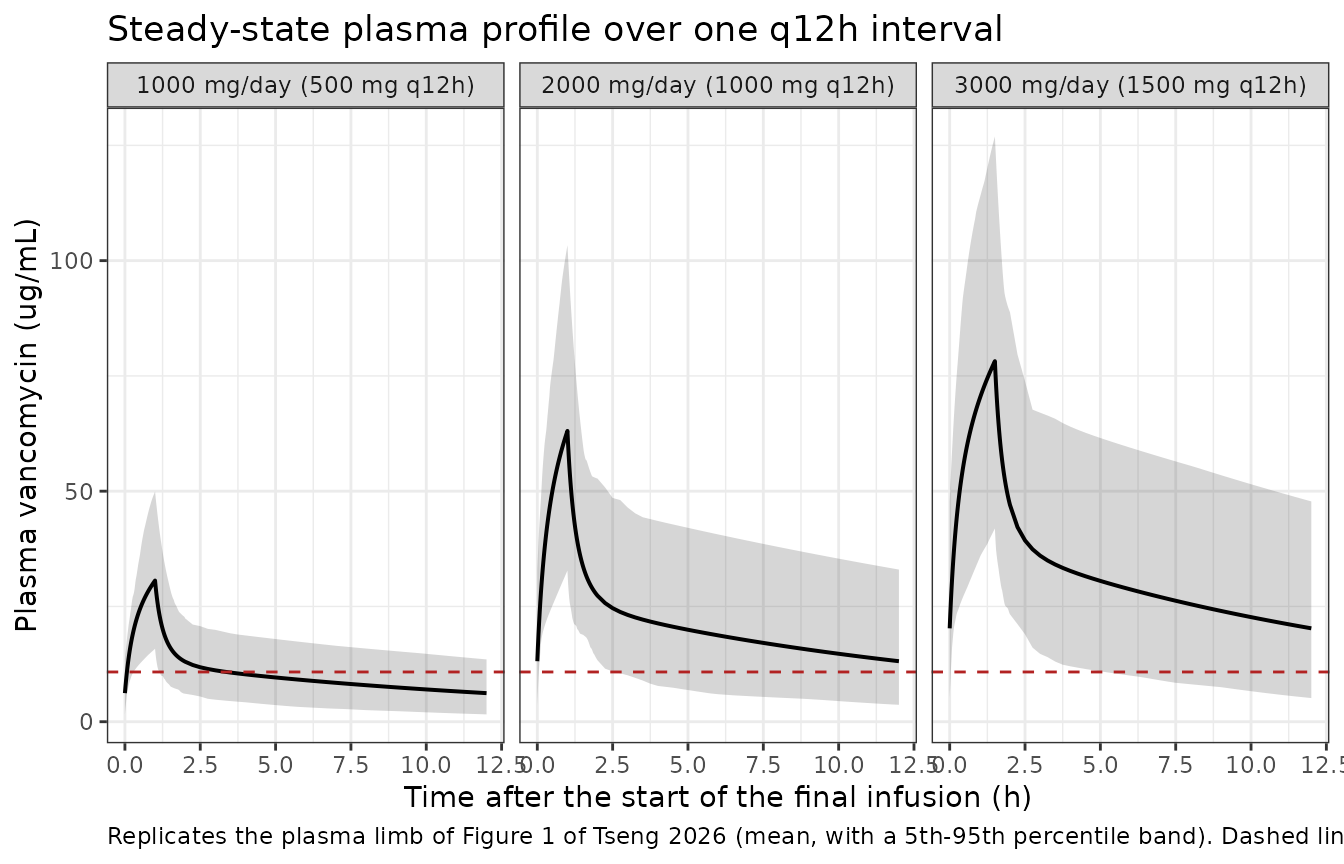

trough_2000 <- sim |>
  filter(arm == "2000 mg/day (1000 mg q12h)", abs(time - ss_end) < 1e-6) |>
  pull(Cc)

c(`Simulated median trough at 2000 mg/day (ug/mL)` = median(trough_2000),
  `Published median plasma trough (ug/mL)`         = 10.79) |>
  round(2)
#> Simulated median trough at 2000 mg/day (ug/mL) 
#>                                           9.98 
#>         Published median plasma trough (ug/mL) 
#>                                          10.79

# The published median pools patients on 1000-3000 mg/day, so this comparison
# is an envelope, not an identity: assert on the CENTRE with generous headroom
# rather than on any extreme. A mis-transcribed clearance or volume moves the
# trough by tens of percent and still breaks this.
stopifnot(abs(median(trough_2000) - 10.79) / 10.79 < 0.60)

PKNCA validation

# Only !is.na(Cc) in this filter: a `time > 0` or `Cc > 0` filter would drop the
# interval-start row PKNCA anchors AUC on.
sim_nca <- sim |>
  dplyr::filter(!is.na(Cc)) |>
  dplyr::select(id, time, Cc, arm)

# Every subject must have a record exactly at the interval start (PKNCA anchors
# AUC there) and at the interval end. The observation grid is constructed to
# contain both, so this asserts rather than patches -- a patch that inserted a
# missing row would hide a broken grid instead of reporting it.
n_subjects <- dplyr::n_distinct(sim_nca$id)
stopifnot(
  nrow(sim_nca) > 0,
  sum(sim_nca$time == ss_start) == n_subjects,
  sum(sim_nca$time == ss_end)   == n_subjects
)

conc_obj <- PKNCA::PKNCAconc(sim_nca, Cc ~ time | arm + id,
                             concu = "ug/mL", timeu = "h")

dose_df <- events |>
  dplyr::filter(evid == 1) |>
  dplyr::transmute(id, arm, time = ss_start, amt = daily_mg)

dose_obj <- PKNCA::PKNCAdose(dose_df, amt ~ time | arm + id, doseu = "mg")

intervals <- data.frame(
  start = ss_start, end = ss_end,
  cmax = TRUE, tmax = TRUE, cmin = TRUE,
  auclast = TRUE, cav = TRUE
)

nca_res <- PKNCA::pk.nca(PKNCA::PKNCAdata(conc_obj, dose_obj, intervals = intervals))
nca_df  <- as.data.frame(nca_res)

nca_df |>
  group_by(arm, PPTESTCD) |>
  summarise(median = median(PPORRES), .groups = "drop") |>
  tidyr::pivot_wider(names_from = PPTESTCD, values_from = median) |>
  knitr::kable(digits = 2,
               caption = "Median steady-state NCA by arm (24 h window, two q12h doses).")

Median steady-state NCA by arm (24 h window, two q12h doses).
arm	auclast	cav	cmax	cmin	tmax
1000 mg/day (500 mg q12h)	243.20	10.13	29.34	5.50	13.0
2000 mg/day (1000 mg q12h)	460.95	19.21	61.94	9.98	13.0
3000 mg/day (1500 mg q12h)	707.60	29.48	72.12	16.10	13.5

# The model is linear, so exposure must scale exactly with dose. This is a
# structural gate on medians (robust), not on any extreme.
auc_by_arm <- nca_df |>
  filter(PPTESTCD == "auclast") |>
  group_by(arm) |>
  summarise(median_auc = median(PPORRES), .groups = "drop") |>
  left_join(distinct(events, arm, daily_mg), by = "arm") |>
  mutate(auc_per_mg = median_auc / daily_mg)

knitr::kable(auc_by_arm, digits = 4,
             caption = "Dose-normalised steady-state AUC0-24 by arm.")

Dose-normalised steady-state AUC0-24 by arm.
arm	median_auc	daily_mg	auc_per_mg
1000 mg/day (500 mg q12h)	243.1990	1000	0.2432
2000 mg/day (1000 mg q12h)	460.9543	2000	0.2305
3000 mg/day (1500 mg q12h)	707.6031	3000	0.2359


# Medians of the same lognormal CL draw across arms differ only by cohort noise.
stopifnot(
  max(auc_by_arm$auc_per_mg) / min(auc_by_arm$auc_per_mg) < 1.15
)

Comparison against published NCA

The paper’s Table 3 medians pool nine patients dosed between 1000 and 3000 mg/day, so the like-for-like simulated comparator is the study-replica cohort, which assigns those nine recovered daily doses in equal proportion.

replica_nca <- sim_replica |>
  dplyr::filter(!is.na(Cc)) |>
  dplyr::mutate(arm = "study replica") |>
  dplyr::select(id, time, Cc, arm)

replica_res <- PKNCA::pk.nca(PKNCA::PKNCAdata(
  PKNCA::PKNCAconc(replica_nca, Cc ~ time | arm + id, concu = "ug/mL", timeu = "h"),
  PKNCA::PKNCAdose(
    events_replica |> filter(evid == 1) |>
      transmute(id, arm = "study replica", time = ss_start, amt = daily_mg),
    amt ~ time | arm + id, doseu = "mg"
  ),
  intervals = data.frame(start = ss_start, end = ss_end,
                         auclast = TRUE, cmax = TRUE, cmin = TRUE, cav = TRUE)
))

# The paper's "trough" is the pre-dose plasma concentration. PKNCA's `ctrough`
# is not usable here (it returns NA for this interval), so `cmin` is used as the
# comparator. That substitution is only valid if the minimum over the 24 h
# window really is the pre-dose concentration -- true at steady state for a
# model that declines monotonically between doses, but asserted rather than
# assumed.
replica_df <- as.data.frame(replica_res)
cmin_by_id <- replica_df |>
  filter(PPTESTCD == "cmin") |>
  transmute(id = as.integer(as.character(id)), cmin = PPORRES)

# (a) Structural, and exactly true: the minimum over the window must fall at one
# of the three pre-dose times, never mid-interval. This is the claim that makes
# cmin a trough. It is cohort-independent and goes red if the profile ever stops
# declining monotonically between doses.
argmin_times <- sim_replica |>
  filter(time >= ss_start, time <= ss_end) |>
  group_by(id) |>
  summarise(t_min = time[which.min(Cc)], .groups = "drop")
stopifnot(all(argmin_times$t_min %in% c(ss_start, ss_start + tau, ss_end)))

# (b) Numerical: cmin and the concentration at the interval end agree to within
# residual accumulation. Realised max 0.02% over this cohort at 30 doses (it was
# 0.21% at 20 doses, driven by the slowest-clearing subjects); 1% admits that
# drift and still goes red on a genuinely non-steady-state window.
cend_by_id <- sim_replica |>
  filter(abs(time - ss_end) < 1e-9) |>
  transmute(id = as.integer(as.character(id)), cend = Cc)
trough_check <- inner_join(cmin_by_id, cend_by_id, by = "id")
stopifnot(
  nrow(trough_check) == 180L,
  max(abs(trough_check$cmin - trough_check$cend) / trough_check$cend) < 0.01
)

published <- tibble::tibble(
  arm     = "study replica",
  auclast = 478.10,   # Table 3, median plasma AUC0-24 (mg*hr/L == ug*hr/mL)
  cmin    = 10.79     # Results, PK Analysis: median plasma trough (ug/mL)
)

cmp <- nlmixr2lib::ncaComparisonTable(
  simulated     = replica_df,
  reference     = published,
  by            = "arm",
  units         = c(auclast = "ug*h/mL", cmin = "ug/mL"),
  tolerance_pct = 20
)

knitr::kable(cmp, caption = paste(
  "Simulated study-replica cohort versus the published Table 3 medians.",
  "* marks a difference above 20%."
), align = c("l", "l", "r", "r", "r"))

Simulated study-replica cohort versus the published Table 3 medians. * marks a difference above 20%.
NCA parameter	arm	Reference	Simulated	% diff
Cmin (ug/mL)	study replica	10.8	11.3	+4.9%
AUClast (ug*h/mL)	study replica	478	492	+2.9%


cmp_num <- as.numeric(gsub("[^0-9.eE+-]", "", cmp$`% diff`))
names(cmp_num) <- cmp[[1]]
round(cmp_num, 1)
#>      Cmin (ug/mL) AUClast (ug*h/mL) 
#>               4.9               2.9

# Cohort-derived and comparing against a nine-patient observed median, so the
# bound is an envelope on the CENTRE. The paper's own patients had individual
# clearances from 2.87 to 13.81 L/h against a typical value of 4.289, so a
# nine-patient median is itself a noisy statistic; 35% admits that without
# admitting a transcription error, which would move AUC by a factor, not a
# fraction.
stopifnot(all(abs(cmp_num) < 35))

Assumptions and deviations

The omega rows of Table 5 are read as variances, not standard deviations. Phoenix NLME prints the Omega matrix in its Random Effect block (variances) and names the residual term separately and explicitly stdev(). Two quantitative checks in the “omega scale” section above agree: the printed relative standard errors (62.6% and 49.4%) match the ~50% expected for a variance from nine subjects rather than the ~25% expected for a standard deviation, and 0.188 read as a variance reproduces the 0.477 log-scale spread of the nine individual clearances in Table 3, whereas read as a standard deviation it is about six-fold too small in variance terms. Both checks are gated so a future re-reading cannot be made silently.
Infusion duration is assumed at 1 hour per gram (minimum 1 hour). Tseng 2026 never reports it, although the model is described as an infusion model and the end-of-infusion concentration is a central result. Every AUC-based gate in this vignette is insensitive to the assumption, because AUC over a steady-state interval is Dose / CL; only the peak and end-of-infusion concentration depend on it, and neither is used as a gate.
Per-patient daily doses are recovered, not published. Tseng 2026 reports only the 1000-3000 mg/day range. The doses simulated here are recovered from Table 3 by Dose(24h) = CL x AUC(0-24), which returns a clean 250 mg multiple for all nine patients (worst case 0.55% off). They are used for the study-replica cohort only; no model parameter depends on them.
No covariates. Tseng 2026 screened twelve (age, sex, disease state, CLcr, eGFR, culture results, CSF WBC, CSF glucose, CSF total protein, cell index, EVD drainage output, urine output) and retained none, attributing this in the Discussion to the dosing nomogram having already adjusted for renal function and to the narrow range of laboratory values in nine patients. The model file therefore has an empty covariateData and records the screened covariates in covariatesDataExcluded (for the seven concepts with a canonical column in this library) and in population$notes (for the six that have none: CSF WBC, CSF glucose, cell index, EVD drainage output, culture results, and the hemorrhage-type disease state). No new canonical covariate column was created for a documentation-only screening entry.
No CSF compartment. The paper’s CSF penetration analysis is noncompartmental plus linear regression on NCA-derived AUCs, not a pharmacokinetic sub-model, and no CSF structural parameter is reported anywhere in the paper. Nothing about CSF is encoded or simulated; the results are tabulated above as source-trace context.
Table 4 versus Table 5. Table 4 reports the same two-compartment model before the covariate search and before the two high-shrinkage random effects were dropped (tvV 6.085, tvCL 4.288, tvCL2 20.157, and additional omega V = 0.011 and omega V2 = 0.000 rows). Table 5 is the final model and is the sole source for every packaged value.
A small central volume. tvV = 6.065 L is low for vancomycin relative to the typical published central volume of roughly 0.2-0.3 L/kg, which makes the distribution half-life about 9 minutes. Vss = tvV + tvV2 = 51.18 L is in the expected range and agrees with the Table 3 median individual volume of 50.46 L to within 1.4%, so the total is well determined and the split between the two compartments is the loosely determined part. This is consistent with a sampling design whose first post-dose sample is at the end of infusion, and with the wide bootstrap interval Table 5 reports for tvV (0.009-19.579 L). Values are used exactly as printed.
Internal inconsistency in the Figure 1 sampling times. The Methods state five samples per interval (pre-dose, end of infusion, and 4, 6 and 8 hours), while the Figure 1 caption lists six (0, 2, 3, 4, 6 and 8 hours). This affects neither the model nor any gate here; it is recorded because it bears on how Figure 1 should be read.
Supplementary material is not on disk. Supplementary Tables S1-S2 and Figures S1-S2 are cited but the EuropePMC supplementary-files endpoint returns HTTP 404 for PMC12965103. None holds a final-model parameter value: S1 is the linear-regression table whose significant rows are reproduced verbatim in the Results text, S2 is the one- versus two- versus three-compartment selection comparison, and S1-S2 figures are diagnostic plots.
cmin stands in for the published trough. The paper reports a median plasma trough concentration; PKNCA’s ctrough returns NA for this interval even with a record at the interval end, so cmin over the 24 hour steady-state window is used as the comparator. The substitution is asserted, not assumed: the chunk above checks that every subject’s minimum falls at one of the three pre-dose times rather than mid-interval (the structural claim that makes cmin a trough at all), and separately that cmin agrees with the concentration at the interval end to within 1%.
Cohort sizes. 150 subjects per dose arm and 20 per recovered dose in the study-replica cohort (180 total), both within the 200-per-arm cap.