Model and source
- Citation: Zhang D, Taylor A, Zhao JJ, Endres CJ, Topletz-Erickson A. Population Pharmacokinetic Analysis of Tucatinib in Healthy Participants and Patients with Breast Cancer or Colorectal Cancer. Clin Pharmacokinet. 2024;63(10):1477-1487. doi:10.1007/s40262-024-01412-0. Correction: Clin Pharmacokinet. 2025;64(1):171-172. doi:10.1007/s40262-024-01458-0 (corrects the Table 2 model-predicted Ctrough,ss geometric mean for mCRC; no final-model parameter in Table 1 is affected).
- Description: Two-compartment population PK model for oral tucatinib (HER2-selective tyrosine kinase inhibitor) in healthy participants and patients with HER2-positive metastatic breast cancer or HER2-positive metastatic colorectal cancer (Zhang 2024, n=283 across seven phase I/II studies). First-order absorption into a depot preceded by an absorption lag time, linear elimination from central, and two-compartment disposition (central + peripheral1). Tumor type is the only covariate retained in the final model: metastatic breast cancer and metastatic colorectal cancer each lower CL relative to the healthy-participant reference, and metastatic colorectal cancer additionally lowers relative bioavailability, so that the net apparent clearance CL/F is 51.9% lower in mBC and 18.7% lower in mCRC. Inter-individual variability on CL and Vc is correlated; Vc carries a very large 135% CV.
- Article: https://doi.org/10.1007/s40262-024-01412-0
- Correction: https://doi.org/10.1007/s40262-024-01458-0
- Supplement (Tables S1-S4, Fig. S1, and the final-model NONMEM control stream): https://doi.org/10.1007/s40262-024-01412-0 (Electronic Supplementary Material, MOESM1 and MOESM2)
Tucatinib is an orally administered, highly selective HER2 tyrosine kinase inhibitor approved at 300 mg twice daily (BID). Zhang 2024 pooled seven phase I/II studies to build a population PK model and to ask whether any clinically relevant covariate warrants a dose adjustment. The answer was no: tumor type was the only covariate retained, and its effect was judged not clinically meaningful.
Population
The analysis dataset contained 3942 quantifiable tucatinib concentrations from 283 participants across seven studies (Table S1): 151 healthy participants (53.4%) from four phase I studies, 63 patients with HER2+ metastatic breast cancer (mBC, 22.3%) from ONT-380-004 and ONT-380-005, and 69 patients with HER2+ metastatic colorectal cancer (mCRC, 24.4%) from the phase II SGNTUC-017 (MOUNTAINEER) study.
Participants had a median age of 48 years (range 18-77), a median body weight of 75.9 kg (range 40.7-146), and 39.9% were female (Tables S2 and S3). Race was 72.4% White, 13.1% Black, 8.8% Asian, with 4.9% missing. Hepatic function was normal in 84.5% and NCI-mild in 14.8%; moderate and severe hepatic impairment, and moderate and severe renal impairment, were not represented in sufficient numbers to be evaluated.
Only fasted marketed-tablet data were used from the healthy-participant studies. HER2CLIMB (ONT-380-206) was excluded because time since the preceding dose was not recorded.
The same information is available programmatically via the model’s
population metadata
(rxode2::rxode(readModelDb("Zhang_2024_tucatinib"))$population).
Model structure
A two-compartment model with linear elimination and first-order
absorption preceded by an absorption lag time (NONMEM
ADVAN4 TRANS4, supplementary control stream). Tumor type
acts on two parameters:
- CL – 51.9% lower in mBC and 70.5% lower in mCRC than in a healthy participant.
- Relative bioavailability (Frel) – 63.7% lower in mCRC only. The mBC effect on Frel was fitted but removed, because it was poorly estimated (RSE 50.4%) and worsened the objective function.
Because both effects act in mCRC and partly offset, the net apparent clearance CL/F is only 18.7% lower in mCRC, while in mBC the full 51.9% reduction carries through. This is the mechanism behind the paper’s headline result: a 2.1-fold AUCss increase in mBC but only a 1.2-fold increase in mCRC, and a lower Cmax in mCRC than in healthy participants.
Source trace
Every ini() entry in
inst/modeldb/specificDrugs/Zhang_2024_tucatinib.R carries
an in-file comment naming its source. They are collected here for
review.
| Equation / parameter | Value | Source location |
|---|---|---|
lcl (CL/F, healthy) |
112 L/h | Table 1, “CL/F (L/h), healthy participants” (4.3% RSE) |
lvc (Vc/F) |
125 L | Table 1, “Vc/F (L)” (11.3% RSE) |
lq (Q/F) |
89.9 L/h | Table 1, “Q/F (L/h)” (5.4% RSE) |
lvp (Vp/F) |
635 L | Table 1, “Vp/F (L)” (4.0% RSE) |
lka (Ka) |
0.424 1/h | Table 1, “Ka (1/h)” (5.3% RSE) |
ltlag (Tlag) |
0.392 h | Table 1, “Tlag (h)” (0.56% RSE) |
lfdepot (Frel, healthy) |
fixed at 1 | Supplementary NONMEM control stream, $PK:
TF1 = 1
|
e_tumtp_breast_cl |
-0.519 | Table 1, “Fractional change in CL/F in participants with HER2+ mBC” (6.3% RSE) |
e_tumtp_crc_cl |
-0.705 | Table 1, “Fractional change in CL/F in participants with HER2+ mCRC” (3.6% RSE) |
e_tumtp_crc_fdepot |
-0.637 | Table 1, “Fractional change in Frel in participants with HER2+ mCRC” (3.8% RSE) |
etalcl variance |
0.184403 | Table 1, “BSV CV CL/F” = 45%; footnote
CV% = sqrt(exp(var) - 1) x 100%
|
etalvc variance |
1.037623 | Table 1, “BSV CV Vc/F” = 135%; same footnote |
etalq variance |
0.176237 | Table 1, “BSV CV Q/F” = 43.9%; same footnote |
etalvp variance |
0.163889 | Table 1, “BSV CV Vp/F” = 42.2%; same footnote |
etalcl/etalvc covariance |
0.205590 | Table 1, “Cov (CL/F, Vc/F)” = 0.470, read as a correlation – see Assumptions and deviations |
addSd |
1.07 ng/mL | Table 1, “Additive residual error SD (ng/mL)” (2.14% RSE) |
propSd |
0.329 | Table 1, “Proportional residual error CV” (0.73% RSE) |
Covariate model form TV * (1 + theta * IND)
|
n/a | Methods 2.2.2 “Categorical” equation; supplementary control stream
$PK CLTUM / F1TUM blocks |
| ODE structure (depot -> central <-> peripheral1) | n/a | Methods 2.2; supplementary control stream
$SUBROUTINE ADVAN4 TRANS4
|
Cc = central / vc * 1000 |
n/a | Supplementary control stream $PK:
S2 = V2/1000 ; dose mg conc ng/mL
|
Closed-form gates on the covariate encoding
Tucatinib disposition is linear, so at steady state the AUC over one
dosing interval has an exact closed form that the paper itself uses
(Methods 2.2.5): AUCss = Dose * Frel / CL. That identity is
an end-to-end check on lcl, lfdepot, and the
tumor-type covariate encoding all at once, and it is independent of the
ODE solver. The asserted values below are computed from the
ini() parameters, then checked against numbers the paper
prints in its text.
tuc <- rxode2::rxode(readModelDb("Zhang_2024_tucatinib"))
#> ℹ parameter labels from comments will be replaced by 'label()'
th  <- setNames(tuc$theta, names(tuc$theta))

cl_healthy <- exp(th[["lcl"]])
frel_ref   <- exp(th[["lfdepot"]])

cl_mbc  <- cl_healthy * (1 + th[["e_tumtp_breast_cl"]])
cl_mcrc <- cl_healthy * (1 + th[["e_tumtp_crc_cl"]])
frel_mcrc <- frel_ref * (1 + th[["e_tumtp_crc_fdepot"]])

dose_mg <- 300
# AUCss in ng*h/mL: (mg / (L/h)) = mg*h/L = ug*h/mL -> x1000 = ng*h/mL
auc_ss <- c(
  Healthy = dose_mg * frel_ref  / cl_healthy,
  mBC     = dose_mg * frel_ref  / cl_mbc,
  mCRC    = dose_mg * frel_mcrc / cl_mcrc
) * 1000

# Net apparent clearance CL/F (what an NCA of these profiles would report)
clf <- dose_mg / (auc_ss / 1000)

tibble::tibble(
  Arm            = names(auc_ss),
  `CL (L/h)`     = c(cl_healthy, cl_mbc, cl_mcrc),
  `Frel`         = c(frel_ref, frel_ref, frel_mcrc),
  `CL/F (L/h)`   = as.numeric(clf),
  `AUCss (ng*h/mL)` = as.numeric(auc_ss),
  `AUCss ratio vs healthy` = as.numeric(auc_ss / auc_ss[["Healthy"]])
) |>
knitr::kable(digits = 3, caption = "Closed-form steady-state exposure implied by the packaged ini() values.")| Arm | CL (L/h) | Frel | CL/F (L/h) | AUCss (ng*h/mL) | AUCss ratio vs healthy |
|---|---|---|---|---|---|
| Healthy | 112.000 | 1.000 | 112.000 | 2678.571 | 1.000 |
| mBC | 53.872 | 1.000 | 53.872 | 5568.756 | 2.079 |
| mCRC | 33.040 | 0.363 | 91.019 | 3296.005 | 1.231 |
These reproduce four separate statements in the paper’s text:
ratio_mbc  <- unname(auc_ss[["mBC"]]  / auc_ss[["Healthy"]])
ratio_mcrc <- unname(auc_ss[["mCRC"]] / auc_ss[["Healthy"]])
clf_drop_mcrc <- 1 - unname(clf[["mCRC"]]) / cl_healthy

# Results 3.5 / Abstract: "2.1-fold" AUCss increase in mBC (90% CI 1.9, 2.3)
stopifnot(abs(ratio_mbc - 2.1) < 0.05, ratio_mbc > 1.9, ratio_mbc < 2.3)
# Results 3.5 / Discussion: "1.2-fold" (Discussion says 1.22) in mCRC (90% CI 1.0, 1.4)
stopifnot(abs(ratio_mcrc - 1.22) < 0.02, ratio_mcrc > 1.0, ratio_mcrc < 1.4)
# Results 3.4: mCRC has "an 18.7% lower CL/F"
stopifnot(abs(clf_drop_mcrc - 0.187) < 0.001)
# Results 3.4: mBC has "51.9% lower clearance"
stopifnot(abs((1 - cl_mbc / cl_healthy) - 0.519) < 1e-9)

c(`AUCss ratio mBC (paper 2.1)`   = ratio_mbc,
  `AUCss ratio mCRC (paper 1.22)` = ratio_mcrc,
  `CL/F reduction mCRC (paper 0.187)` = clf_drop_mcrc)
#>       AUCss ratio mBC (paper 2.1)     AUCss ratio mCRC (paper 1.22)
#>                         2.0790021                         1.2305085
#> CL/F reduction mCRC (paper 0.187)
#>                         0.1873278
A second, independent gate: the apparent steady-state volume.
Vss/F is (Vc/F + Vp/F) / Frel, which the model
makes 760 L in healthy participants and mBC, but
760 / 0.363 = 2094 L in mCRC. Table 2 reports median Vss/F
of 752 L (healthy), 838 L (mBC) and 2130 L (mCRC) – the
mCRC value confirms that Frel divides the apparent volumes exactly as
encoded.
vss_f <- c(Healthy = (exp(th[["lvc"]]) + exp(th[["lvp"]])) / frel_ref,
           mBC     = (exp(th[["lvc"]]) + exp(th[["lvp"]])) / frel_ref,
           mCRC    = (exp(th[["lvc"]]) + exp(th[["lvp"]])) / frel_mcrc)
# Table 2 (corrected) median Vss/F for mCRC = 2130 L
stopifnot(abs(vss_f[["mCRC"]] - 2130) / 2130 < 0.05)
round(vss_f, 1)
#> Healthy     mBC    mCRC
#>   760.0   760.0  2093.7
Virtual cohort
Original participant-level data are not public. The cohorts below are 200 participants per arm, dosed 300 mg BID – the approved regimen and the regimen Table 2 tabulates. The only covariates the final model uses are the two tumor-type indicators, so each arm is defined entirely by them; a healthy participant is the reference (both indicators 0).
Seven days of BID dosing is more than five effective half-lives for every arm (the paper reports effective half-lives of 11.9 h in mBC and 16.4 h in mCRC), so the final interval is at steady state. A washout follows the last dose so that the terminal half-life can be estimated; the washout window is scaled to each arm’s own half-life, because a single shared window would fit the fast (healthy) arm’s terminal slope to solver noise.
set.seed(20240808)

n_per_arm <- 200L
tau       <- 12      # h, BID
n_doses   <- 14L     # 7 days
t_lastdose <- tau * (n_doses - 1L)   # 156 h
t_ss_end   <- t_lastdose + tau       # 168 h

arms <- tibble::tribble(
  ~treatment,  ~TUMTP_BREAST, ~TUMTP_CRC, ~washout_h, ~id_offset,
  "Healthy",   0,             0,          48,         0L,
  "HER2+ mBC", 1,             0,          72,         1000L,
  "HER2+ mCRC", 0,            1,          120,        2000L
)

make_cohort <- function(treatment, TUMTP_BREAST, TUMTP_CRC, washout_h, id_offset,
                        n = n_per_arm) {
  subj <- tibble::tibble(
    id           = id_offset + seq_len(n),
    treatment    = treatment,
    TUMTP_BREAST = TUMTP_BREAST,
    TUMTP_CRC    = TUMTP_CRC
  )
  obs_times <- sort(unique(c(
    seq(0, tau, by = 0.25),                              # dense first interval
    seq(tau, t_lastdose, by = tau),                      # troughs in between
    seq(t_lastdose, t_ss_end, by = 0.25),                # dense steady-state interval
    seq(t_ss_end, t_ss_end + washout_h, by = 2)          # washout, arm-specific
  )))
  doses <- subj |>
    tidyr::crossing(time = seq(0, t_lastdose, by = tau)) |>
    dplyr::mutate(amt = dose_mg, evid = 1L, cmt = "depot")
  obs <- subj |>
    tidyr::crossing(time = obs_times) |>
    dplyr::mutate(amt = NA_real_, evid = 0L, cmt = "central")
  dplyr::bind_rows(doses, obs) |>
    dplyr::arrange(id, time, dplyr::desc(evid))
}

events <- dplyr::bind_rows(lapply(seq_len(nrow(arms)), function(i) {
  do.call(make_cohort, as.list(arms[i, ]))
}))

# Disjoint IDs across arms are mandatory: rxSolve treats id as the subject key,
# and duplicated ids across cohorts silently merge into one subject.
stopifnot(!anyDuplicated(unique(events[, c("id", "time", "evid")])))
stopifnot(dplyr::n_distinct(events$id) == 3L * n_per_arm)
Simulation
Between-subject variability on Vc/F is 135% CV. At that magnitude the
default LSODA solver silently returns NA for a substantial
minority of subjects, so dop853 is used throughout.
mod <- readModelDb("Zhang_2024_tucatinib")

sim <- rxode2::rxSolve(
  mod,
  events = events,
  keep   = c("treatment", "TUMTP_BREAST", "TUMTP_CRC"),
  method = "dop853"
) |>
  as.data.frame()
#> ℹ parameter labels from comments will be replaced by 'label()'

# Guard against the silent all-NA / partial-NA solver failure mode.
stopifnot(mean(is.na(sim$Cc)) < 0.001)
Cc is the individual prediction (IPRED). Table 2 of the
paper reports model-predicted exposures from post-hoc
parameters, so IPRED – not the residual-error-perturbed sim
column – is the right comparator.
A deterministic typical-value profile is simulated alongside,
matching the paper’s own approach in Methods 2.2.5 (“using typical
model-estimated PK parameters without including between-subject
variability”). Setting the eta columns to zero in the event table and
passing omega = NA is preferred over zeroRe(),
which mutates the shared model object.
events_typ <- events |>
  dplyr::filter(id %% 1000L == 1L) |>   # one representative subject per arm
  dplyr::mutate(etalcl = 0, etalvc = 0, etalq = 0, etalvp = 0)

sim_typ <- rxode2::rxSolve(
  mod,
  events = events_typ,
  keep   = c("treatment"),
  omega  = NA,
  method = "dop853"
) |>
  as.data.frame()
#> Warning: multi-subject simulation without without 'omega'

stopifnot(dplyr::n_distinct(sim_typ$treatment) == 3L)
Replicated figures
Steady-state concentration-time profiles
sim_typ |>
  dplyr::filter(time >= t_lastdose, time <= t_ss_end) |>
  dplyr::mutate(tad = time - t_lastdose) |>
  ggplot(aes(tad, Cc, colour = treatment)) +
  geom_line(linewidth = 0.8) +
  labs(x = "Time after dose (h)", y = "Tucatinib concentration (ng/mL)",
       colour = NULL,
       title = "Typical-value steady-state profile, 300 mg BID",
       caption = "Compare with the steady-state exposures tabulated in Table 2 of Zhang 2024.") +
  theme_bw()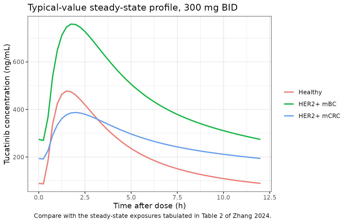
The ordering reproduces the paper’s central finding: mBC sits well above healthy across the whole interval, whereas mCRC has a lower peak than healthy participants but a higher trough – the signature of reduced bioavailability combined with reduced clearance.
Figure 2 – prediction-corrected VPC (cohort spread)
sim |>
  dplyr::filter(time >= t_lastdose, time <= t_ss_end) |>
  dplyr::mutate(tad = time - t_lastdose) |>
  dplyr::group_by(treatment, tad) |>
  dplyr::summarise(
    Q05 = quantile(Cc, 0.05, na.rm = TRUE),
    Q50 = quantile(Cc, 0.50, na.rm = TRUE),
    Q95 = quantile(Cc, 0.95, na.rm = TRUE),
    .groups = "drop"
  ) |>
  ggplot(aes(tad, Q50)) +
  geom_ribbon(aes(ymin = Q05, ymax = Q95), alpha = 0.25, fill = "steelblue") +
  geom_line(linewidth = 0.8) +
  facet_wrap(~treatment) +
  scale_y_log10() +
  labs(x = "Time after dose (h)", y = "Tucatinib concentration (ng/mL)",
       title = "Simulated steady-state spread (median, 5th-95th percentile)",
       caption = "Analogous to the prediction-corrected VPC in Figure 2 of Zhang 2024.") +
  theme_bw()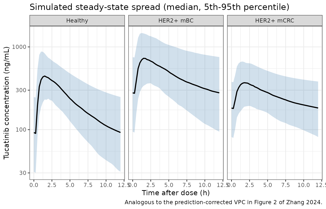
Figure 3 – clearance stratified by tumor type
Figure 3 of the paper plots model-predicted CL/F in the two patient groups and reports geometric means of 53.4 L/h (mBC) and 89.0 L/h (mCRC).
clf_ind <- sim |>
  dplyr::group_by(id, treatment) |>
  dplyr::summarise(clf = mean(cl / fdepot), .groups = "drop")

gm <- clf_ind |>
  dplyr::group_by(treatment) |>
  dplyr::summarise(`Geometric mean CL/F (L/h)` = exp(mean(log(clf))), .groups = "drop")

knitr::kable(gm, digits = 1,
caption = "Replicates Figure 3 of Zhang 2024 (published geometric means: 53.4 L/h mBC, 89.0 L/h mCRC).")| treatment | Geometric mean CL/F (L/h) |
|---|---|
| HER2+ mBC | 53.4 |
| HER2+ mCRC | 95.3 |
| Healthy | 111.5 |
# These are sampling estimates, not exact identities: the geometric mean of a
# log-normal CL converges to its typical value (53.87 and 91.02 L/h here), but
# with n = 200 the mean of the etas still has an SD of sqrt(0.1844/200) = 0.030,
# so a few percent of drift either way is expected. The 10% band accommodates
# that while still catching a mis-encoded covariate effect.
gm_v <- setNames(gm[[2]], gm[[1]])
stopifnot(abs(gm_v[["HER2+ mBC"]]  - 53.4) / 53.4 < 0.10)
stopifnot(abs(gm_v[["HER2+ mCRC"]] - 89.0) / 89.0 < 0.10)

clf_ind |>
  dplyr::filter(treatment != "Healthy") |>
  ggplot(aes(treatment, clf)) +
  geom_boxplot(outlier.alpha = 0.3, width = 0.5) +
  scale_y_log10() +
  labs(x = NULL, y = "Model-predicted CL/F (L/h)",
       title = "Figure 3 - tucatinib clearance stratified by tumor type",
       caption = "Replicates Figure 3 of Zhang 2024.") +
  theme_bw()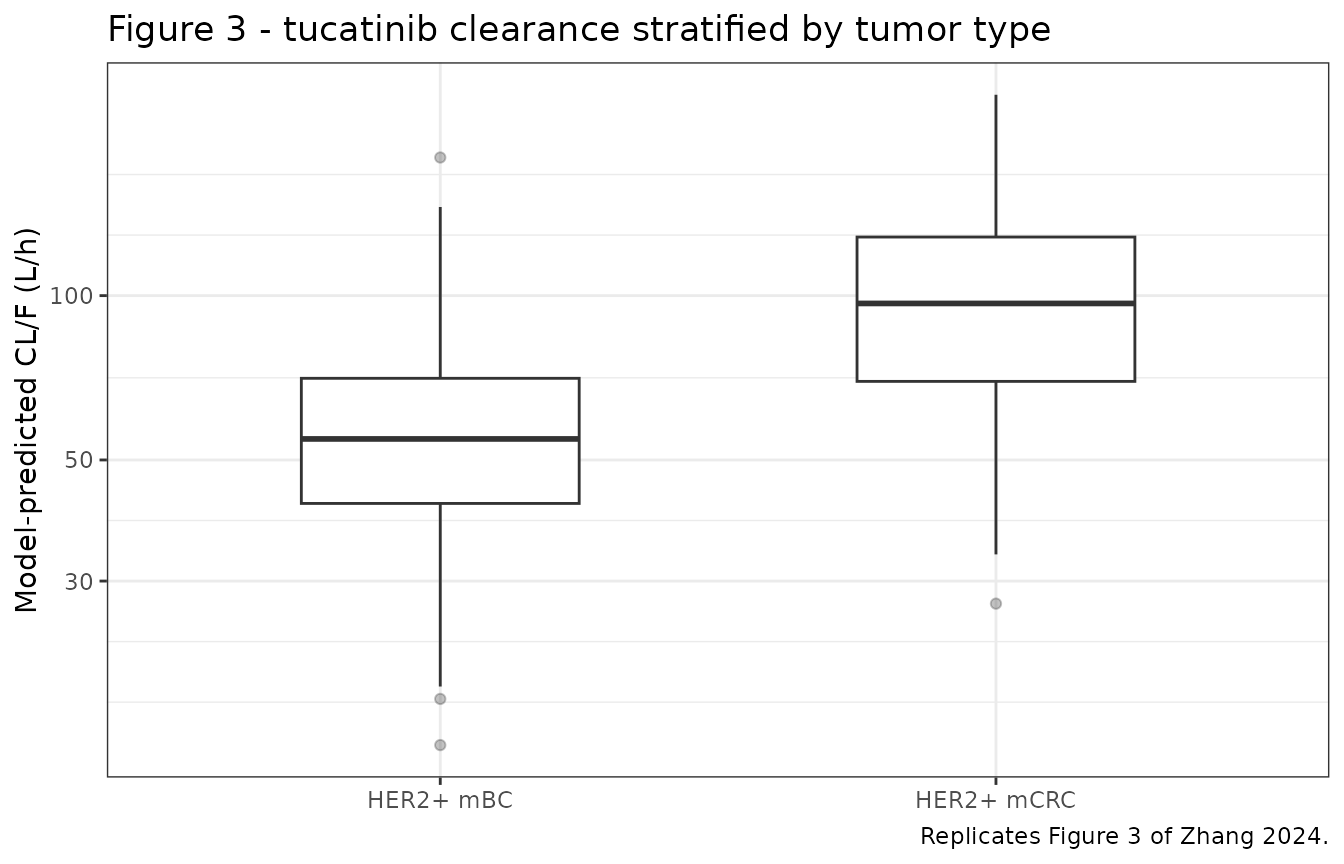
PKNCA validation
NCA is run on the simulated individual predictions over three intervals per arm: the first dosing interval (for accumulation ratios), the final dosing interval (steady state), and an arm-specific post-dose washout window (terminal half-life).
sim_nca <- sim |>
  dplyr::filter(!is.na(Cc)) |>
  dplyr::select(id, time, Cc, treatment)

# Guarantee a time-zero record per subject; pre-dose Cc = 0 for an
# extravascular dose. Without it PKNCA warns once per subject that the AUC
# range starts before the first measurement.
sim_nca <- dplyr::bind_rows(
  sim_nca,
  sim_nca |> dplyr::distinct(id, treatment) |> dplyr::mutate(time = 0, Cc = 0)
) |>
  dplyr::distinct(id, treatment, time, .keep_all = TRUE) |>
  dplyr::arrange(id, treatment, time)

dose_df <- events |>
  dplyr::filter(evid == 1) |>
  dplyr::select(id, time, amt, treatment)

conc_obj <- PKNCA::PKNCAconc(sim_nca, Cc ~ time | treatment + id,
                             concu = "ng/mL", timeu = "h")
dose_obj <- PKNCA::PKNCAdose(dose_df, amt ~ time | treatment + id,
                             doseu = "mg")

blank <- function(...) {
  base <- list(cmax = FALSE, tmax = FALSE, cmin = FALSE,
               auclast = FALSE, cav = FALSE, half.life = FALSE)
  base[names(list(...))] <- list(...)
  base
}

intervals <- dplyr::bind_rows(
  # first dosing interval - denominator of the accumulation ratios
  tibble::tibble(treatment = arms$treatment, start = 0, end = tau) |>
    dplyr::bind_cols(tibble::as_tibble(blank(cmax = TRUE, auclast = TRUE))),
  # final dosing interval - steady state
  tibble::tibble(treatment = arms$treatment, start = t_lastdose, end = t_ss_end) |>
    dplyr::bind_cols(tibble::as_tibble(blank(cmax = TRUE, tmax = TRUE, cmin = TRUE,
                                             auclast = TRUE, cav = TRUE))),
  # arm-specific washout - terminal half-life
  tibble::tibble(treatment = arms$treatment, start = t_ss_end,
                 end = t_ss_end + arms$washout_h) |>
    dplyr::bind_cols(tibble::as_tibble(blank(half.life = TRUE)))
)

nca_res <- PKNCA::pk.nca(PKNCA::PKNCAdata(conc_obj, dose_obj, intervals = intervals))
nca_df  <- as.data.frame(nca_res)
# Interval filtering matters: cmax and auclast are requested on two different
# intervals, so pooling without filtering would silently average the first-dose
# and steady-state values.
ss   <- nca_df |> dplyr::filter(start == t_lastdose)
fst  <- nca_df |> dplyr::filter(start == 0)
term <- nca_df |> dplyr::filter(start == t_ss_end, PPTESTCD == "half.life")

# Trough concentrations are read directly at the exact end-of-interval grid
# times rather than via PKNCA. `cmin` over the FIRST interval would return the
# pre-dose zero at t = 0, not the 12 h trough, so it is not usable as the
# accumulation-ratio denominator. Reading the concentration at a grid point is
# a lookup, not an NCA calculation, so no inline trapezoidal work is involved.
troughs <- sim |>
  dplyr::filter(time %in% c(tau, t_ss_end)) |>
  dplyr::mutate(which = ifelse(time == tau, "first", "ss")) |>
  dplyr::select(treatment, id, which, Cc) |>
  tidyr::pivot_wider(names_from = which, values_from = Cc) |>
  dplyr::mutate(PPTESTCD = "ctrough")

stopifnot(nrow(troughs) == 3L * n_per_arm, !anyNA(troughs$first), !anyNA(troughs$ss))

# Accumulation ratios: steady state over first dose, per subject.
rac <- dplyr::bind_rows(
  dplyr::inner_join(
    ss  |> dplyr::filter(PPTESTCD %in% c("auclast", "cmax")) |>
      dplyr::select(treatment, id, PPTESTCD, ss = PPORRES),
    fst |> dplyr::filter(PPTESTCD %in% c("auclast", "cmax")) |>
      dplyr::select(treatment, id, PPTESTCD, first = PPORRES),
    by = c("treatment", "id", "PPTESTCD")
  ),
  troughs |> dplyr::select(treatment, id, PPTESTCD, ss, first)
) |>
  dplyr::mutate(rac = ss / first)

rac_summary <- rac |>
  dplyr::group_by(treatment, PPTESTCD) |>
  dplyr::summarise(Median = median(rac, na.rm = TRUE), .groups = "drop") |>
  tidyr::pivot_wider(names_from = PPTESTCD, values_from = Median) |>
  dplyr::rename("Rac, AUC" = auclast, "Rac, Cmax" = cmax, "Rac, Ctrough" = ctrough,
                "Arm" = treatment)

knitr::kable(rac_summary, digits = 2,
caption = "Simulated median accumulation ratios at 300 mg BID. Published (Table 2 medians): Rac AUC 1.34 / 1.94 / 2.45; Rac Cmax 1.19 / 1.59 / 1.92; Rac Ctrough 1.57 / 2.38 / 2.96 for healthy / mBC / mCRC.")| Arm | Rac, AUC | Rac, Cmax | Rac, Ctrough |
|---|---|---|---|
| HER2+ mBC | 1.83 | 1.53 | 2.20 |
| HER2+ mCRC | 2.27 | 1.84 | 2.88 |
| Healthy | 1.34 | 1.21 | 1.61 |
Comparison against the published NCA
Table 2 of Zhang 2024 (as amended by the 2024 correction) tabulates
model-predicted steady-state exposures at 300 mg BID. The medians are
transcribed below and compared against the simulated cohort;
ncaComparisonTable() pools the per-subject simulated values
by median, which matches the published statistic.
sim_long <- dplyr::bind_rows(
  ss   |> dplyr::filter(PPTESTCD %in% c("cmax", "auclast")) |>
    dplyr::select(treatment, id, PPTESTCD, PPORRES),
  term |> dplyr::filter(PPTESTCD == "half.life") |>
    dplyr::select(treatment, id, PPTESTCD, PPORRES),
  troughs |> dplyr::transmute(treatment, id, PPTESTCD, PPORRES = ss)
)

# Table 2 medians [min, max] as published; the correction of 2024-12-11 revised
# only the mCRC Ctrough,ss geometric mean (405 -> 197), leaving the medians as
# originally printed.
published <- tibble::tribble(
  ~treatment,   ~auclast, ~cmax, ~ctrough, ~half.life,
  "Healthy",     2730,     480,   88.4,     8.76,
  "HER2+ mBC",   5770,     759,   303,      16.2,
  "HER2+ mCRC",  3230,     402,   188,      21.3
)

cmp <- nlmixr2lib::ncaComparisonTable(
  simulated = sim_long,
  reference = published,
  by        = "treatment",
  units     = c(cmax = "ng/mL", ctrough = "ng/mL",
                auclast = "ng*h/mL", half.life = "h"),
  tolerance_pct = 20
)

knitr::kable(cmp,
             caption = "Simulated vs. published model-predicted steady-state NCA (Zhang 2024 Table 2 medians). * differs by >20%.",
align = c("l", "l", "r", "r", "r"))| NCA parameter | treatment | Reference | Simulated | % diff |
|---|---|---|---|---|
| Cmax (ng/mL) | Healthy | 480 | 467 | -2.7% |
| Cmax (ng/mL) | HER2+ mBC | 759 | 755 | -0.6% |
| Cmax (ng/mL) | HER2+ mCRC | 402 | 377 | -6.2% |
| AUClast (ng*h/mL) | Healthy | 2730 | 2730 | -0.1% |
| AUClast (ng*h/mL) | HER2+ mBC | 5770 | 5490 | -4.8% |
| AUClast (ng*h/mL) | HER2+ mCRC | 3230 | 3100 | -4.1% |
| t½ (h) | Healthy | 8.76 | 9.38 | +7.1% |
| t½ (h) | HER2+ mBC | 16.2 | 14.7 | -9.2% |
| t½ (h) | HER2+ mCRC | 21.3 | 21.2 | -0.5% |
| Ctrough (ng/mL) | Healthy | 88.4 | 92.4 | +4.5% |
| Ctrough (ng/mL) | HER2+ mBC | 303 | 279 | -8.0% |
| Ctrough (ng/mL) | HER2+ mCRC | 188 | 183 | -2.8% |
attr(cmp, "footnote")
#> NULL
# Regression guard, computed from the raw values rather than by parsing the
# formatted table (the friendly labels are unicode, e.g. "t<half>", so string
# matching on them is brittle). All four parameters across all three arms hold
# inside the same 20% band that ncaComparisonTable() stars on -- the observed
# worst case is -9.2% (mBC half-life), so 20% leaves roughly 2x headroom for
# solver/platform drift without letting a mis-encoded covariate effect through.
sim_med <- sim_long |>
  dplyr::group_by(treatment, PPTESTCD) |>
  dplyr::summarise(sim = median(PPORRES, na.rm = TRUE), .groups = "drop")

ref_long <- published |>
  tidyr::pivot_longer(-treatment, names_to = "PPTESTCD", values_to = "ref")

chk <- dplyr::inner_join(sim_med, ref_long, by = c("treatment", "PPTESTCD")) |>
  dplyr::mutate(`% diff` = (sim - ref) / ref * 100)

stopifnot(nrow(chk) == 12L)   # 3 arms x 4 parameters, all matched
stopifnot(all(abs(chk$`% diff`) < 20))

chk |> dplyr::arrange(PPTESTCD, treatment) |> knitr::kable(digits = 1)| treatment | PPTESTCD | sim | ref | % diff |
|---|---|---|---|---|
| HER2+ mBC | auclast | 5491.2 | 5770.0 | -4.8 |
| HER2+ mCRC | auclast | 3097.9 | 3230.0 | -4.1 |
| Healthy | auclast | 2726.3 | 2730.0 | -0.1 |
| HER2+ mBC | cmax | 754.7 | 759.0 | -0.6 |
| HER2+ mCRC | cmax | 376.9 | 402.0 | -6.2 |
| Healthy | cmax | 467.2 | 480.0 | -2.7 |
| HER2+ mBC | ctrough | 278.7 | 303.0 | -8.0 |
| HER2+ mCRC | ctrough | 182.7 | 188.0 | -2.8 |
| Healthy | ctrough | 92.4 | 88.4 | 4.5 |
| HER2+ mBC | half.life | 14.7 | 16.2 | -9.2 |
| HER2+ mCRC | half.life | 21.2 | 21.3 | -0.5 |
| Healthy | half.life | 9.4 | 8.8 | 7.1 |
Assumptions and deviations
-
Cov (CL/F, Vc/F) = 0.470in Table 1 is encoded as a correlation, not a covariance. Table 1’s BSV block reports variability on the normalised CV% scale, with the footnoteBSV CV% = sqrt(exp(variance) - 1) x 100%. Applying that footnote gives variances of 0.184403 (CL/F, 45%) and 1.037623 (Vc/F, 135%). Reading 0.470 as a covariance would imply a correlation of0.470 / sqrt(0.184403 * 1.037623) = 1.074, i.e. an Omega that is not positive semi-definite and thatrxSolvecannot Cholesky-decompose. The largest covariance the reported CVs admit is 0.4429, even at the extremes of their rounding intervals, so the covariance reading is arithmetically excluded rather than merely unlikely. A correlation of 0.470 is feasible and is consistent with the rest of the Table 1 BSV block being reported on the normalised scale. The encoded covariance is therefore0.470 * sqrt(0.184403 * 1.037623) = 0.205590. The footnote’s CV formula is independently corroborated by the supplementary control stream’s$OMEGAinitial estimates (0.15 -> 40.2% and 0.99 -> 130.0%, adjacent to the final 45% and 135%). -
A second, uncorrected inconsistency in Table 2. The
mCRC
Vss/Fcolumn gives a median of 2130 L [1680, 4690] but a geometric mean of 829 L (20.9% CV). A geometric mean cannot sit that far below the minimum of its own range. The model reproduces the median (2094 L, i.e. 760 L divided by the mCRC Frel of 0.363) and not the geometric mean, which suggests the geometric mean was computed without the Frel division. The published correction of 2024-12-11 addressed only the mCRCCtrough,ssgeometric mean and did not touch this cell. No model parameter depends on it. -
Terminal half-life. Simulated median terminal
half-lives agree with the published medians to within 10% in all three
arms (+7.1% healthy, -9.2% mBC, -0.5% mCRC), so
half.lifeis held to the same 20% band as the exposure metrics. The residual spread is expected rather than structural: Table 2’s half-lives are computed from post-hoc individual parameters, and the 135% CV on Vc/F makes the distribution of individual terminal slopes wide, so the median of a 200-subject sample need not land exactly on the published median of a 52- to 128-subject one. The washout window is scaled per arm so that each arm’s terminal slope is fitted over a comparable number of its own half-lives. No parameter was tuned. - Absorption rate. The paper notes a median observed Tmax of 1-2 h after a single 300 mg dose, but the popPK Ka of 0.424 1/h (absorption half-life 1.6 h) yields a later simulated Tmax. The authors discuss this directly: the popPK Ka is a pooled compromise across highly variable absorption profiles, and agrees with the independent PBPK estimate (Tlag 0.5 h, Ka 0.6 1/h). The value is used as published.
-
Covariates screened but not retained. Body weight,
sex, race, age, albumin, creatinine clearance, ECOG performance status
and NCI hepatic dysfunction category were all tested and dropped during
backward elimination. They are recorded in the model file’s
covariatesDataExcludedmetadata so the provenance of the covariate search is preserved without declaring covariates thatmodel()never references. - Virtual cohort covariates. Because the final model uses only the two tumor-type indicators, no demographic distributions had to be assumed; each arm is fully specified by its indicator pair. Arm sizes are 200 per arm rather than the published 128 / 52 / 68, which changes only the sampling precision of the simulated medians.
- Regimen. All arms are simulated at 300 mg BID, the approved dose and the regimen Table 2 tabulates. The 50 mg and 150 mg BID arms of SGNTUC-015 and the 350 mg BID minority in ONT-380-004/005 are not simulated; tucatinib disposition is linear in the model, so those arms scale proportionally.
-
New canonical covariate column.
TUMTP_CRCwas added toinst/references/covariate-columns.mdas part of this extraction. It is a well-formed member of the existingTUMTP_<type>family and is the sister indicator explicitly anticipated by theTUMTP_BREASTentry.