Paclitaxel whole-body PBPK, mouse and human (Fu 2019)
Source:vignettes/articles/Fu_2019_paclitaxel_pbpk.Rmd
Fu_2019_paclitaxel_pbpk.RmdModel and source
- Citation: Fu Q, Sun X, Lustberg MB, Sparreboom A, Hu S. Predicting Paclitaxel Disposition in Humans With Whole-Body Physiologically-Based Pharmacokinetic Modeling. CPT Pharmacometrics Syst Pharmacol. 2019;8(12):931-939.
- Article: https://doi.org/10.1002/psp4.12472 (open access, PMC6930855)
- Supplement: Table S1 (mouse and human physiology) and Code S1 (the Phoenix PML code “for the final PBPK model”, with a mouse block and a human block).
Fu et al. built a whole-body PBPK model for paclitaxel given in its Cremophor EL formulation (Taxol). They fitted it to their own tissue distribution data in female FVB mice, then scaled it to a 70-kg adult and compared it against plasma profiles from 14 cancer patients who received 175 mg/m^2 as a 3-h infusion. The package ships the two models as separate files:
-
Fu_2019_paclitaxel_mouse_pbpk: 30-g mouse physiology; partition coefficients, CLint and PS from Table 1. -
Fu_2019_paclitaxel_human_pbpk: 70-kg adult physiology; all parameters from the human block of Code S1.
Both models share one topology. Venous blood flows through the lung,
which sits in series, into arterial blood. Arterial blood perfuses eight
flow-limited tissues: spleen, liver, kidney, heart, gut, muscle, fat and
brain. It also perfuses a permeability-limited remainder with a vascular
+ interstitial subspace (is_remainder) and an intracellular
subspace (int_remainder). Spleen and gut drain into the
liver. Hepatic metabolism, fu * CLint * C_liver / Kp_liver,
is the only route of elimination, and the plasma unbound fraction is
fixed at 0.05. The dose goes into venous blood (Code S1
Dosepoint(Ab)), and the observed plasma concentration is
the arterial pool (Code S1 Cp = Ca).
mod_mouse <- readModelDb("Fu_2019_paclitaxel_mouse_pbpk")
mod_human <- readModelDb("Fu_2019_paclitaxel_human_pbpk")
Population
Mouse. The mice were female FVB, 10-14 weeks old and
weighing 23-29 g (the Methods give an average of 25 g). Each received a
single 20 mg/kg IV bolus of Taxol diluted to 3 mg/mL. Four animals were
killed at each of 0.5, 1, 4, 8 and 24 h. The model physiology is that of
a 30-g reference mouse (Table S1; Code S1 BW = 0.03).
Human. The patients were 14 adults (> 18 years) with confirmed solid tumors. Each received single-agent paclitaxel at 175 mg/m^2 as a 3-h infusion, with plasma sampled out to 21 h after the end of the infusion (Methods; van Zuylen 2001). The model physiology is that of a 70-kg reference adult. The paper does not give demographics beyond these.
The same information is available as
mod_mouse()$population and
mod_human()$population.
Source trace
| Quantity | Mouse value | Human value | Source |
|---|---|---|---|
| ODE structure (13 states) | – | – | Code S1 deriv() statements; paper Eqs. 1-7 |
| Blood split venous / arterial | 0.75 / 0.25 of blood volume | same | Code S1 Vbla, Vblb
|
| Remainder split vascular+ISF / cell | 0.333 / 0.667 | same | Code S1 Vrv, Vre
|
Organ volume fractions fv_*
|
Code S1 mouse FV_*
|
Code S1 human FV_*
|
Code S1; volumes match Table S1 |
Cardiac output co
|
885 mL/h | 394.6 L/h | Code S1 CO (394600 mL/h for the human) |
Flow fractions fq_*
|
Code S1 mouse FQ_*
|
Code S1 human FQ_*
|
Code S1; flows match Table S1 |
fu |
0.05 (fixed) | 0.05 (fixed) | Methods; Code S1 |
kp_spleen |
0.83 | 0.833372 | Table 1 / Code S1 human tvKs
|
kp_liver |
2.8 | 2.82516 | Table 1 / tvKl
|
kp_kidney |
1 | 1.01274 | Table 1 / tvKk
|
kp_heart |
0.54 | 0.541566 | Table 1 / tvKh
|
kp_lung |
0.77 | 0.778136 | Table 1 / tvKlu
|
kp_gut |
1.61 | 1.62708 | Table 1 / tvKg
|
kp_muscle |
0.37 | 0.37604 | Table 1 / tvKm
|
kp_adipose |
0.58 | 0.586303 | Table 1 / tvKf
|
kp_brain |
0.03 | 0.035072 | Table 1 / tvKbr
|
kp_remainder (Code S1 Kr) |
0.52 | 0.527921 | Table 1 Kr / tvKr
|
kp_int_remainder (Code S1 Krt) |
2.63 | 2.60612 | Table 1 K_ISF / tvKrt
|
ps_remainder |
43 mL/h | 61.7295 L/h | Table 1 PS r / tvPSr = 61729.5 mL/h |
clint |
79.72 mL/h | 449.886 L/h | Table 1 Cl int,H / tvCll = 449886
mL/h |
propSd |
0.218255 | 0.252886 | Code S1 CEps2 (mouse / human block) |
Mouse model
Simulation
Dose: 20 mg/kg for the 25-g average mouse the Methods describe, i.e. 500 ug as an IV bolus into venous blood. The model contains no inter-individual variability, so a single typical-value solve is enough.
dose_mouse <- 20 * 25 # ug (20 mg/kg x 0.025 kg)
ev_mouse <- et(amt = dose_mouse, cmt = "venous") |>
  et(seq(0, 24, by = 0.05), cmt = "venous")
sim_mouse <- as.data.frame(rxSolve(mod_mouse, ev_mouse, returnType = "data.frame"))

organ_cols <- c(
  plasma = "Cc", spleen = "c_spleen", liver = "c_liver", kidney = "c_kidney",
  heart = "c_heart", lung = "c_lung", gut = "c_gut", muscle = "c_muscle",
  fat = "c_adipose", brain = "c_brain"
)
mouse_long <- sim_mouse |>
  select(time, all_of(organ_cols)) |>
  pivot_longer(-time, names_to = "organ", values_to = "conc") |>
  mutate(id = 1L, organ = factor(organ, levels = names(organ_cols)))
Replicates Figure 4 (mouse plasma and tissues)
ggplot(filter(mouse_long, time > 0), aes(time, conc)) +
  geom_line(colour = "darkgreen") +
  scale_y_log10() +
  facet_wrap(~organ, scales = "free_y", ncol = 5) +
  labs(
    x = "Time (h)", y = "Paclitaxel concentration (ug/mL)",
    caption = "Replicates the model lines of Figure 4 of Fu 2019 (20 mg/kg IV bolus in mice)."
  ) +
  theme_bw()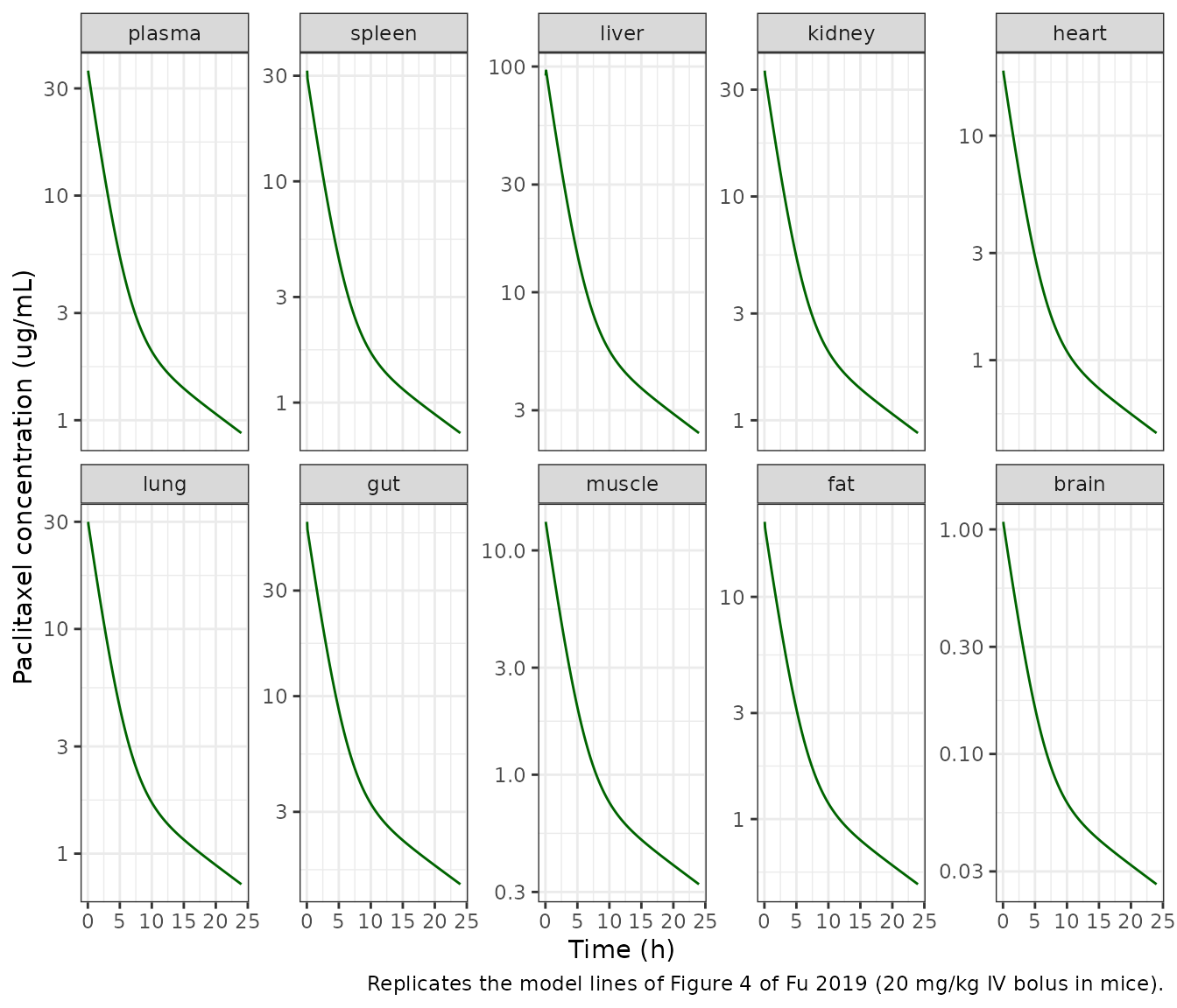
PKNCA: AUC(0-24) against Table 2
Table 2 of Fu 2019 lists AUC(0-last) for plasma and nine tissues, both from NCA of the observed data and from the PBPK predictions. The last sampling time was 24 h.
conc_obj <- PKNCAconc(mouse_long, conc ~ time | organ + id)
dose_df <- data.frame(organ = factor(names(organ_cols), levels = names(organ_cols)), id = 1L, time = 0, amt = dose_mouse)
dose_obj <- PKNCAdose(dose_df, amt ~ time | organ + id, route = "intravascular")
intervals <- data.frame(start = 0, end = 24, auclast = TRUE, cmax = TRUE)
nca_mouse <- pk.nca(PKNCAdata(conc_obj, dose_obj, intervals = intervals))

table2 <- data.frame(
  organ = names(organ_cols),
  auclast_pbpk = c(104.55, 130.85, 365.79, 137.84, 56.09, 87.19, 169.42, 39.35, 61.22, 3.63),
  auclast_nca = c(106.08, 115.13, 379.04, 138.83, 52.45, 82.75, 139.98, 40, 65.03, 3.38)
)

sim_auc <- as.data.frame(nca_mouse$result) |>
  filter(PPTESTCD == "auclast") |>
  mutate(organ = as.character(organ)) |>
  select(organ, PPTESTCD, PPORRES)

cmp_pbpk <- ncaComparisonTable(
  sim_auc,
  transmute(table2, organ, auclast = auclast_pbpk),
  by = "organ",
  units = c(auclast = "h*ug/mL")
)
knitr::kable(cmp_pbpk, caption = "Simulated AUC(0-24) vs Table 2 'PBPK estimated' (Fu 2019).")| NCA parameter | organ | Reference | Simulated | % diff |
|---|---|---|---|---|
| AUClast (h*ug/mL) | plasma | 105 | 110 | +5.2% |
| AUClast (h*ug/mL) | spleen | 131 | 91.9 | -29.8%* |
| AUClast (h*ug/mL) | liver | 366 | 302 | -17.6% |
| AUClast (h*ug/mL) | kidney | 138 | 110 | -20.0%* |
| AUClast (h*ug/mL) | heart | 56.1 | 59.4 | +6.0% |
| AUClast (h*ug/mL) | lung | 87.2 | 91.7 | +5.2% |
| AUClast (h*ug/mL) | gut | 169 | 178 | +5.2% |
| AUClast (h*ug/mL) | muscle | 39.4 | 41.1 | +4.4% |
| AUClast (h*ug/mL) | fat | 61.2 | 64.3 | +5.0% |
| AUClast (h*ug/mL) | brain | 3.63 | 3.3 | -9.1% |
Differences above 20% are starred. Plasma, heart, lung, gut, muscle, fat and brain all fall within about 10% of the paper’s own PBPK predictions. Spleen, liver and kidney come out about 18-30% below them. The cause is inside the paper, not in this model. For a perfusion-limited organ the tissue-to-plasma AUC ratio equals that organ’s Kp (see the check below). In Table 2 the ratio is 1.25 for spleen, 3.50 for liver and 1.32 for kidney, but the Table 1 estimates are 0.83, 2.8 and 1.0. Table 1’s own “NCA estimated” Kp column (0.73, 2.74, 1.03) is also inconsistent with the Table 2 NCA AUC ratios (1.09, 3.57, 1.31) for exactly the same three organs. The other seven organs agree between the two tables.
auc <- setNames(sim_auc$PPORRES, sim_auc$organ)
kp_table1 <- c(heart = 0.54, gut = 1.61, muscle = 0.37, fat = 0.58, brain = 0.03)
ratio_sim <- auc[names(kp_table1)] / auc[["plasma"]]
ratio_tab2 <- setNames(table2$auclast_pbpk, table2$organ)[names(kp_table1)] / 104.55
knitr::kable(data.frame(
  organ = names(kp_table1),
  "Kp (Table 1)" = kp_table1,
  "AUC ratio, simulated" = signif(ratio_sim, 3),
  "AUC ratio, Table 2 PBPK" = signif(ratio_tab2, 3),
  check.names = FALSE
), row.names = FALSE, caption = "Tissue:plasma AUC(0-24) ratio vs Kp.")| organ | Kp (Table 1) | AUC ratio, simulated | AUC ratio, Table 2 PBPK |
|---|---|---|---|
| heart | 0.54 | 0.540 | 0.5360 |
| gut | 1.61 | 1.620 | 1.6200 |
| muscle | 0.37 | 0.373 | 0.3760 |
| fat | 0.58 | 0.585 | 0.5860 |
| brain | 0.03 | 0.030 | 0.0347 |
stopifnot(
  # Flow-limited organs: AUC ratio tracks Kp (truncation at 24 h only)
  all(abs(ratio_sim / kp_table1 - 1) < 0.05),
  # ...and reproduces the paper's own PBPK ratios for these organs; brain is
  # compared loosely because Table 1 prints Kbr to one significant figure
  all(abs(ratio_sim[c("heart", "gut", "muscle", "fat")] / ratio_tab2[c("heart", "gut", "muscle", "fat")] - 1) < 0.05),
  # Plasma AUC(0-24) vs Table 2 PBPK (104.55 h*ug/mL)
  abs(auc[["plasma"]] / 104.55 - 1) < 0.10
)
Mass balance
The paper’s arterial and venous blood-flow bookkeeping is not
balanced. For the mouse, q_lung = 0.814 CO, while the flows
written out of the arterial pool add up to
(1 - fq_spleen - fq_gut) CO = 0.881 CO. The equations still
conserve drug mass, because every flux leaving one state enters another.
With CLint set to (practically) zero, total body drug amount must
therefore stay at the dose.
states <- c(
  "venous", "lung", "arterial", "spleen", "liver", "is_remainder",
  "int_remainder", "kidney", "heart", "muscle", "adipose", "gut", "brain"
)
mb <- as.data.frame(rxSolve(mod_mouse, ev_mouse, params = c(lclint = log(1e-10))))
total <- rowSums(mb[, states])
stopifnot(max(abs(total / dose_mouse - 1)) < 1e-4)
range(total)
#> [1] 500 500
Human model
Simulation against Figure 3
Dose: 175 mg/m^2 as a 3-h infusion. The paper does not give the patients’ body surface area, so 1.8 m^2 is assumed (a 70-kg reference adult), for 315 mg. The observed means below were digitised from Figure 3 of Fu 2019 (times measured from the start of infusion).
bsa <- 1.8
dose_human <- 175 * bsa # mg
obs_fig3 <- data.frame(
  time = c(1, 2, 3, 3.25, 3.5, 4, 4.25, 5, 7, 11, 13, 24),
  conc = c(1.6, 2.8, 4.0, 3.6, 2.8, 1.8, 1.15, 0.7, 0.42, 0.2, 0.135, 0.068)
)
ev_human <- et(amt = dose_human, dur = 3, cmt = "venous") |>
  et(sort(unique(c(seq(0, 24, by = 0.05), obs_fig3$time))), cmt = "venous")
sim_human <- as.data.frame(rxSolve(mod_human, ev_human, returnType = "data.frame"))

# Methods text alternative: 'The CLint used in the human simulation was set to
# a value of 1,410 L/hour'
sim_text <- as.data.frame(rxSolve(mod_human, ev_human, params = c(lclint = log(1410)), returnType = "data.frame"))

pred <- rbind(
  data.frame(time = sim_human$time, conc = sim_human$Cc, variant = "Code S1 (CLint 449.9 L/h, packaged)"),
  data.frame(time = sim_text$time, conc = sim_text$Cc, variant = "Methods text (CLint 1,410 L/h)")
)
ggplot(filter(pred, time > 0), aes(time, conc, colour = variant)) +
  geom_line() +
  geom_point(data = obs_fig3, aes(time, conc), inherit.aes = FALSE) +
  scale_y_log10() +
  labs(
    x = "Time since start of infusion (h)", y = "Plasma paclitaxel (mg/L)", colour = NULL,
    caption = "Replicates Figure 3 / Figure 5b of Fu 2019 (points: digitised observed means, n = 14)."
  ) +
  theme_bw() +
  theme(legend.position = "bottom")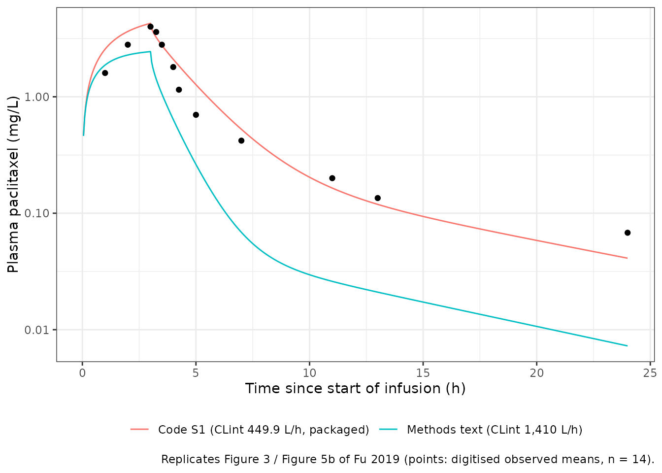
at_obs <- function(s) approx(s$time, s$Cc, xout = obs_fig3$time)$y
log_err_code <- log(at_obs(sim_human) / obs_fig3$conc)
log_err_text <- log(at_obs(sim_text) / obs_fig3$conc)
c(
  rms_log_error_code = sqrt(mean(log_err_code^2)),
  rms_log_error_text = sqrt(mean(log_err_text^2))
)
#> rms_log_error_code rms_log_error_text
#>          0.3247291          1.3148401
stopifnot(
  # Packaged (Code S1) parameters follow the observed means (typical-value
  # model vs digitised means; the residual SD is 0.25 on the natural scale)
  sqrt(mean(log_err_code^2)) < 0.5,
  abs(median(log_err_code)) < 0.3,
  # The CLint quoted in the Methods text is off by more than 3-fold in RMS
  sqrt(mean(log_err_text^2)) > 3 * sqrt(mean(log_err_code^2))
)
PKNCA: plasma NCA against the digitised Figure 3 means
The paper gives no human NCA table, so the reference is PKNCA run on the digitised observed means, treated as one profile. The pre-dose sample is taken as zero.
nca_one <- function(df, label) {
  df <- df |> mutate(id = 1L, treatment = label)
  cobj <- PKNCAconc(df, conc ~ time | treatment + id)
  dobj <- PKNCAdose(
    data.frame(treatment = label, id = 1L, time = 0, amt = dose_human, dur = 3),
    amt ~ time | treatment + id,
    route = "intravascular", duration = "dur"
  )
  iv <- data.frame(start = 0, end = 24, cmax = TRUE, tmax = TRUE, auclast = TRUE)
  pk.nca(PKNCAdata(cobj, dobj, intervals = iv))
}
obs_nca_input <- bind_rows(data.frame(time = 0, conc = 0), obs_fig3)
sim_nca_input <- sim_human |>
  filter(!is.na(Cc)) |>
  filter(time %in% obs_nca_input$time) |>
  transmute(time, conc = Cc)
nca_obs <- nca_one(obs_nca_input, "175 mg/m2 3-h infusion")
nca_sim <- nca_one(sim_nca_input, "175 mg/m2 3-h infusion")

ref_wide <- as.data.frame(nca_obs$result) |>
  select(treatment, PPTESTCD, PPORRES) |>
  pivot_wider(names_from = PPTESTCD, values_from = PPORRES)
cmp_human <- ncaComparisonTable(
  nca_sim, ref_wide,
  by = "treatment",
  units = c(cmax = "mg/L", tmax = "h", auclast = "h*mg/L")
)
knitr::kable(cmp_human, caption = "Simulated (Code S1 human block) vs digitised Figure 3 NCA, sampled at the Figure 3 times.")| NCA parameter | treatment | Reference | Simulated | % diff |
|---|---|---|---|---|
| Cmax (mg/L) | 175 mg/m2 3-h infusion | 4 | 4.27 | +6.8% |
| Tmax (h) | 175 mg/m2 3-h infusion | 3 | 3 | +0.0% |
| AUClast (h*mg/L) | 175 mg/m2 3-h infusion | 14 | 16.9 | +20.6%* |
Both profiles are sampled at the Figure 3 times, so the two NCAs share the same trapezoidal error. Cmax and Tmax agree. AUC(0-24) is about 20% above the digitised reference (starred). Most of the excess comes from the rising limb and the first two hours after the infusion ends (1-5 h), where the model runs above the observed means; Cmax and the terminal phase agree. Two inputs of the comparison are uncertain and may account for part of this. The BSA of 1.8 m^2 is assumed; the dose, and so the AUC, scales linearly with it. The reference itself was digitised by eye from a log-scale figure. The parameters were not tuned.
Replicates Figure 5a (predicted human tissue profiles)
human_long <- sim_human |>
  select(time, all_of(organ_cols)) |>
  pivot_longer(-time, names_to = "organ", values_to = "conc") |>
  mutate(organ = factor(organ, levels = names(organ_cols)))
ggplot(filter(human_long, time > 0), aes(time, conc)) +
  geom_line(colour = "steelblue") +
  scale_y_log10() +
  facet_wrap(~organ, scales = "free_y", ncol = 5) +
  labs(
    x = "Time since start of infusion (h)", y = "Paclitaxel concentration (mg/L)",
    caption = "Typical-value analogue of Figure 5a of Fu 2019 (175 mg/m^2, 3-h infusion)."
  ) +
  theme_bw()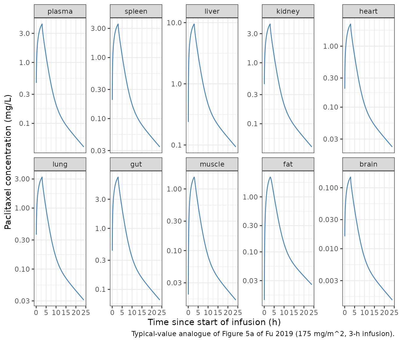
Assumptions and deviations
-
Two parameter sources, one per species. Code S1 has
a mouse block and a human block. The mouse block’s
fixef()values (e.g. Ks 1.027, Kl 3.34, CLint 93.1 mL/h, PSr 64, Krt 4) do not match the final mouse estimates in Table 1. Its PSr = 64 and Krt = 4 are round numbers, which suggests initial values rather than estimates. The mouse model therefore uses Table 1, the paper’s reported final estimates with CV% and CIs. Simulated plasma AUC(0-24) with Table 1 is about 6% above Table 2; with the Code S1 mouse block it is within 5% for a 600-ug dose but 13% low for 500 ug. Table 1 also reproduces the Table 2 tissue/plasma ratios for heart, gut, muscle, fat and brain; the Code S1 mouse block does not. The human model uses the Code S1 human block, which is the only complete human parameter set the paper provides. -
Human CLint. The Methods say “The CL int used in
the human simulation was set to a value of 1,410 L/hour”, but Code S1
has
tvCll = 449886mL/h (449.9 L/h). The Figure 3 comparison above settles it: 449.9 L/h follows the observed means (RMS log error about 0.3), while 1,410 L/h predicts a profile that collapses after the infusion. The packaged value is 449.9 L/h. -
Remainder partition coefficients. The printed Eqs.
3-4 call the flow-side coefficient
K_ISFand the intracellular-side coefficientKpt. Table 1 listsKr = 0.52andK_ISF = 2.63. Code S1 usesKron the flow side andKrton the intracellular side, and its human block values (0.528, 2.606) match Table 1’sKrandK_ISFrespectively. The model follows Code S1:kp_remainder = Kr,kp_int_remainder = K_ISF. The swapped mapping moves plasma AUC(0-24) 17% above Table 2 instead of 6%. -
Liver equation sign. Printed Eq. 2 adds the liver
outflow term (
+ Ql * Cl / Kl); Code S1 subtracts it. The model uses the Code S1 sign. The printed sign would not conserve mass. - Blood-flow bookkeeping. Arterial outflow and lung/cardiac inflow do not balance (see Mass balance). This is reproduced exactly as in Code S1, not corrected.
-
Residual error. Code S1 applies one proportional
error (
CEps2) to the plasma and every tissue observation. The packaged models declare only the plasma endpointCc ~ prop(propSd); tissue concentrations are algebraic outputs (c_<organ>). The mousepropSdcomes from the Code S1 mouse block, the only mouse value reported. - No IIV. Fu 2019 reports no between-subject variances. The Phoenix predictive check “included” variability on the Kp’s, PSr and CLint, but no values are given, so both models are typical-value models.
-
Mouse dose and weight. The physiology is for a 30-g
mouse (Code S1
BW = 0.03, Table S1), while the Methods give an average weight of 25 g. The vignette doses 20 mg/kg x 25 g = 500 ug. - Human dose. BSA is not reported; 1.8 m^2 is assumed (315 mg).
- Figure data. The human plasma means were digitised by eye from Figure 3. They are approximate, and the gate thresholds allow for that.