Belantamab mafodotin M-protein tumor growth inhibition (Collins 2023) • nlmixr2lib

Model and source

Citation: Collins J, van Noort M, Rathi C, Post TM, Struemper H, Jewell RC, Ferron-Brady G. Longitudinal efficacy and safety modeling and simulation framework to aid dose selection of belantamab mafodotin for patients with multiple myeloma. CPT Pharmacometrics Syst Pharmacol. 2023;12(10):1411-1424. doi:10.1002/psp4.13016. The two-compartment PK structure originates with Struemper et al. (2019) and is re-estimated in Collins 2023 Table S1; the full covariate population PK model for the same drug is available as modellib(‘Papathanasiou_2025_belantamab’).
Description: Concentration-driven tumor growth inhibition (TGI) model for serum M-protein in patients with relapsed/refractory multiple myeloma treated with the antibody-drug conjugate belantamab mafodotin, with logistic growth plus a modified weak Allee term, a saturating effect-compartment driven kill term, an exponential resistance decay, and covariate effects of baseline beta-2-microglobulin on the growth rate, baseline M-protein on the kill rate, and extramedullary disease plus baseline soluble BCMA on the effect-compartment rate constant (Collins 2023). The embedded two-compartment time-varying-clearance PK layer is a typical-value ADC driver taken from Collins 2023 Table S1; for the full covariate population PK model of belantamab mafodotin see modellib(‘Papathanasiou_2025_belantamab’). The paper’s ocular-safety discrete time Markov model is not included (see vignette).
Article: https://doi.org/10.1002/psp4.13016 (open access)
Supplement (Tables S1-S2, Figures S1-S3): https://doi.org/10.1002/psp4.13016, Appendix S1

Collins 2023 builds an integrated efficacy / safety simulation framework for belantamab mafodotin, an anti-BCMA antibody-drug conjugate (ADC) carrying the microtubule-disrupting payload monomethyl auristatin F (MMAF). The framework has three components:

a two-compartment population PK model with sigmoidal time-varying clearance (Collins 2023 Table S1; re-estimated from the model originally published by Struemper et al.),
a concentration-driven tumor growth inhibition (TGI) model for the time course of serum M-protein, the plasma-cell-burden marker used to assess response in multiple myeloma (Collins 2023 Figure 1a and Table 1), and
a discrete time Markov model (DTMM) for the time course of ocular event grades on the GSK Keratopathy and Visual Acuity (KVA) scale (Collins 2023 Figure 1b and Table 1).

This vignette covers component 2, the M-protein TGI model, which is what the packaged Collins_2023_belantamab_mprotein model file implements, together with a typical-value version of component 1 embedded as the ADC concentration driver. Components 1 and 3 are out of scope for this file; see Assumptions and deviations below for the reasoning and for the cross-reference to the full covariate population PK model, Papathanasiou_2025_belantamab.

Model structure

The M-protein state tumor holds the serum M-protein concentration in g/L. The equations are printed verbatim in Collins 2023 Figure 1a:

$\frac{dM(t)}{dt} = \mathrm{KGR}'(t)\,M(t) - \mathrm{KD}'(t)\,M(t)$

$\mathrm{KGR}'(t) = \mathrm{KGR}\cdot\frac{M(t)}{M(t) + A_{50}}\cdot\left(1 - \frac{M(t)}{150}\right)$

$\mathrm{KD}'(t) = \mathrm{KD}\cdot\left(1 - e^{-\mathrm{Slope}\cdot C}\right)\cdot e^{-\lambda t}$

where $C$ is the effect-site ADC concentration (Collins 2023 abbreviation list: “C, effect concentration”), obtained from a Sheiner-type effect compartment driven by the plasma ADC concentration with rate constant KEO:

$\frac{dC}{dt} = \mathrm{KEO}\cdot\left(C_c - C\right)$

Three features distinguish this from a plain exponential-kill TGI model:

the logistic factor $(1 - M/150)$ enforces a carrying capacity of 150 g/L, fixed from the literature so that unrealistic M-protein values are never simulated;
the modified weak Allee factor $M/(M + A_{50})$ slows growth at very low M-protein concentrations, consistent with cooperative-growth models of tumours (50% growth reduction at $M = A_{50} = 1.16$ g/L); and
the kill term saturates in exposure via $1 - e^{-\mathrm{Slope}\cdot C}$ rather than being linear in concentration, and decays with an exponential resistance term $e^{-\lambda t}$ .

Population

The M-protein model was estimated from 169 patients with relapsed/refractory multiple myeloma: 42 from the phase I dose-escalation study DREAMM-1 (0.03-4.6 mg/kg every 3 weeks) and 127 from the pivotal phase II study DREAMM-2 (2.5 and 3.4 mg/kg every 3 weeks). Only patients who were followed for response by serum M-protein and who had a baseline M-protein concentration $\ge$ 5 g/L entered the dataset (Collins 2023 Results, M-protein).

Collins 2023 does not tabulate demographics for that 169-patient estimation subset; per-study baseline characteristics are reported only in the primary DREAMM-1 and DREAMM-2 publications. What Collins 2023 does report (Table S2) is the baseline distribution of the 218-patient DREAMM-2 simulation population, which retained its model-building covariate values:

Characteristic	Mean (SD)	Median (5th, 95th percentile)
Weight (kg)	76.2 (17.3)	73.3 (53.0, 108)
Albumin (g/L)	38.3 (4.76)	39 (30, 45)
$\beta_2$ -microglobulin (nmol/L)	470 (431)	364 (170, 1034)
Soluble BCMA (ng/mL)	173 (244)	88.2 (6.28, 587)
M-protein (g/L)	18.5 (15.6)	13.0 (3.0, 50.3)

The virtual cohort below is built to approximate these four marginal distributions. The same information is available programmatically via readModelDb("Collins_2023_belantamab_mprotein")()$population.

Source trace

The per-parameter origin is recorded as an in-file comment next to each ini() entry in inst/modeldb/specificDrugs/Collins_2023_belantamab_mprotein.R. The table below collects them in one place for review.

Equation / parameter	Value	Source location
`d/dt(tumor) <- (kgr_t - kd_t) * tumor`	n/a	Figure 1a, `dM(t)/dt` equation
`kgr_t <- kg * tumor/(tumor + a50) * (1 - tumor/tsmax)`	n/a	Figure 1a, `KGR'(t)` equation
`kd_t <- kd * (1 - exp(-slope * effect)) * exp(-lambda * t)`	n/a	Figure 1a, `KD'(t)` equation
`d/dt(effect) <- ke0 * (Cc - effect)`	n/a	Figure 1a schematic (KEO into the effect compartment); abbreviation list “C, effect concentration”
`lkg` (TVKGR)	0.0174 /day (95% CI 0.0146, 0.0208)	Table 1
`lkd` (TVKD)	0.0207 /day (95% CI 0.0159, 0.0268)	Table 1
`llambda` (TVLAMBDA)	0.0024 /day (95% CI 0.00123, 0.00480)	Table 1
`lslope` (Slope)	0.619 mL/ug (95% CI 0.554, 0.691)	Table 1
`lke0` (TVKEO)	0.0284 /day (95% CI 0.0248, 0.0326)	Table 1
`la50` (A50)	1.16 g/L (95% CI 0.839, 1.481)	Table 1 value; unit from Methods text (“50% growth reduction at M-protein < 1.16 g/L”) – see Errata
`ltsmax` (carrying capacity)	150 g/L, `fixed()`	Methods (“carrying capacity fixed at 150 g/L based on existing literature”); also printed in the Figure 1a `KGR'(t)` equation
`e_b2m_kg`	0.219 (95% CI 0.011, 0.427)	Table 1 “Effect of bB2M on KGR”; equation `KGRpop = TVKGR*(bB2M/350)^theta`
`e_mcprot_kd`	1.41 (95% CI 1.08, 1.85)	Table 1 “Effect of bMPROT < 20 on KD”; equation `KDpop = TVKD*theta`
`e_emd_ke0`	0.108 (95% CI 0.0617, 0.187)	Table 1 “Effect of MEDFL on KEO”; equation `KEOpop = TVKEOtheta_Extramedullary(sBCMA/100)^theta`
`e_sbcma_ke0`	-0.414 (95% CI -0.561, -0.267)	Table 1 “Effect of baseline sBCMA on KEO”
`etalkg`, `etalkd`, `etallambda` 3x3 block	0.677 / 0.546 / 1.07 / 0.217 / 1.12 / 3.04	Table 1 random-effects rows (omega^2 KGR, Cov(KGR~KD), omega^2 KD, Cov(KGR~LAMBDA), Cov(KD~LAMBDA), omega^2 LAMBDA)
`etalke0`	`fixed(0.015)`	Table 1 “omega^2 KEO FIXED”
`etalslope`	`fixed(0.015)`	Table 1 “omega^2 Slope fixed”
`etala50`	`fixed(0.015)`	Table 1 “omega^2 A50 fixed”
`propSd_tumor`	0.0633 (%RSE 6.2)	Table 1 “%RES ERR, proportional”
`addSd_tumor`	0.832 g/L (%RSE 3.8)	Table 1 “%RES ERR, additive SD”
`lcl` (TVCL)	0.915 L/day	Table S1
`lvc` (TVV1)	4.46 L	Table S1
`lq` (TVQ)	0.740 L/day	Table S1
`lvp` (TVV2)	6.49 L	Table S1
`cl_hill_max` (IMAX)	-0.309	Table S1
`lcl_hill_t50` (TI50)	56.9 days	Table S1
`cl_hill_gamma` (Gamma)	3.81	Table S1
`propSd` (ADC residual)	0.026	Table S1 “RES ERR, additive sigma on log scale”
B2M reference 350 nmol/L	n/a	Table 1 `KGRpop` equation
SBCMA reference 100 ng/mL	n/a	Table 1 `KEOpop` equation
bMPROT threshold 20 g/L	n/a	Table 1 row label “Effect of bMPROT < 20 on KD”
Simulation horizon 315 days, q3w assessments	n/a	Methods, Simulation
Response definition (>= 50% M-protein reduction)	n/a	Methods, Simulation (IMWG partial response)
Regimen ORR ratios	see Table 2 replication below	Table 2

Virtual cohort

Original observed data are not publicly available. The cohort below draws the four model covariates from log-normal distributions matched to the Collins 2023 Table S2 medians and 5th-95th percentiles, and assigns extramedullary disease with a 24% prevalence (the DREAMM-2 figure; Collins 2023 itself does not report the MEDFL prevalence – see Errata).

Cohort size is 150 participants per arm, below the 200-per-arm cap.

set.seed(20230713)

n_per_arm <- 150L

# Log-normal parameters matched to the Table S2 medians and 5th-95th
# percentiles: median = exp(mu); the 5th-95th span gives
# sigma = log(p95 / p05) / (2 * 1.6449).
lnorm_from_median_span <- function(median, p05, p95) {
  c(mu = log(median), sigma = log(p95 / p05) / (2 * stats::qnorm(0.95)))
}

par_wt     <- lnorm_from_median_span(73.3, 53.0, 108)
par_b2m    <- lnorm_from_median_span(364,  170,  1034)
par_sbcma  <- lnorm_from_median_span(88.2, 6.28, 587)
par_mcprot <- lnorm_from_median_span(13.0, 3.0,  50.3)

# Helper: one arm's covariate table. `id_offset` keeps ids disjoint across
# arms so rxSolve never merges two subjects into one.
make_cohort <- function(n, arm, id_offset = 0L) {
  tibble::tibble(
    id      = id_offset + seq_len(n),
    arm     = arm,
    WT      = stats::rlnorm(n, par_wt[["mu"]],     par_wt[["sigma"]]),
    B2M     = stats::rlnorm(n, par_b2m[["mu"]],    par_b2m[["sigma"]]),
    SBCMA   = stats::rlnorm(n, par_sbcma[["mu"]],  par_sbcma[["sigma"]]),
    MCPROT  = stats::rlnorm(n, par_mcprot[["mu"]], par_mcprot[["sigma"]]),
    DIS_EMD = stats::rbinom(n, 1L, 0.24)
  ) |>
    # Entry criterion: baseline M-protein >= 5 g/L (Collins 2023 Results).
    dplyr::mutate(MCPROT = pmax(MCPROT, 5))
}

# Helper: build several arms and bind them, asserting that subject ids stay
# disjoint. rxSolve treats id as the subject key, so a collision across arms
# would silently merge two subjects into one that receives the summed dose.
map_arms_bind <- function(x, f) {
  out <- dplyr::bind_rows(Map(f, x, seq_along(x)))
  stopifnot(!anyDuplicated(unique(out[, c("id", "time", "evid")])))
  out
}

Dosing regimens

Collins 2023 Table 2 lists eleven simulated regimens. Six of them use a fixed schedule with no ocular-event-driven dose reduction, and those are the ones this vignette can reproduce without the DTMM (see Errata). Doses are in mg/kg and are converted to mg with each subject’s weight.

# Each regimen is a list of (time in days, dose in mg/kg) dosing events over
# the paper's 315-day simulation horizon.
horizon_d <- 315

q3w <- seq(0, horizon_d - 1, by = 21)
q1w <- seq(0, horizon_d - 1, by = 7)

regimens <- list(
  `2.5 mg/kg q3w (reference)` =
    tibble::tibble(time = q3w, mgkg = 2.5),
  `1.4 mg/kg q3w` =
    tibble::tibble(time = q3w, mgkg = 1.4),
  `0.9 mg/kg q3w` =
    tibble::tibble(time = q3w, mgkg = 0.9),
  `1.25 mg/kg D1 + D8 q3w (split)` =
    tibble::tibble(
      time = sort(c(q3w, q3w + 7)),
      mgkg = 1.25
    ),
  `0.83 mg/kg qw (metronomic)` =
    tibble::tibble(time = q1w, mgkg = 0.83),
  `2.5 mg/kg q3w, step down to 1.9 at D21` =
    tibble::tibble(time = q3w, mgkg = ifelse(q3w >= 21, 1.9, 2.5))
)

# M-protein was assessed every 3 weeks (Collins 2023 Methods).
obs_times_eff <- seq(0, horizon_d, by = 21)

build_arm_events <- function(cov_tbl, sched) {
  doses <- cov_tbl |>
    tidyr::crossing(sched) |>
    dplyr::mutate(
      amt  = WT * mgkg,
      evid = 1L,
      cmt  = "central",
      dur  = 1 / 24            # 1-hour IV infusion (assumption; see Errata)
    ) |>
    dplyr::select(-mgkg)
  obs <- cov_tbl |>
    tidyr::crossing(time = obs_times_eff) |>
    dplyr::mutate(
      amt  = NA_real_,
      evid = 0L,
      # `tumor` is both an ODE state and a declared endpoint, so it is a valid
      # observation cmt for this two-endpoint model. rxode2 returns the
      # algebraic ADC observable `Cc` as a column on the same rows.
      cmt  = "tumor",
      dur  = NA_real_
    )
  dplyr::bind_rows(doses, obs) |>
    dplyr::arrange(id, time, dplyr::desc(evid)) |>
    as.data.frame()
}

events_eff <- map_arms_bind(regimens, function(sched, k) {
  build_arm_events(
    make_cohort(n_per_arm, names(regimens)[k],
                id_offset = (k - 1L) * n_per_arm),
    sched
  )
})

c(rows = nrow(events_eff), subjects = dplyr::n_distinct(events_eff$id))
#>     rows subjects 
#>    34650      900

Simulation

mod <- readModelDb("Collins_2023_belantamab_mprotein")

sim_eff <- rxode2::rxSolve(
  mod,
  events = events_eff,
  keep   = c("arm", "WT", "B2M", "SBCMA", "MCPROT", "DIS_EMD")
) |>
  as.data.frame()
#> ℹ parameter labels from comments will be replaced by 'label()'

# The published simulations resampled individual variability for every
# replication, so the population solve must actually vary. This assertion
# guards against a silently zeroed OMEGA (see the zeroRe() note in Errata).
stopifnot(stats::sd(log(sim_eff$kg)) > 0.3)

Replicate published figures

Figure 2a – M-protein concentration-time profiles

Collins 2023 Figure 2a is a goodness-of-fit panel of observed and model-predicted serum M-protein against time from first dose, spanning roughly 0-300 days on the x-axis and 0-120 g/L on the y-axis. The panel below shows the simulated median and 5th-95th percentile band for the reference 2.5 mg/kg q3w regimen on the same axes.

sim_eff |>
  dplyr::filter(arm == "2.5 mg/kg q3w (reference)") |>
  dplyr::group_by(time) |>
  dplyr::summarise(
    Q05 = stats::quantile(tumor, 0.05, na.rm = TRUE),
    Q50 = stats::quantile(tumor, 0.50, na.rm = TRUE),
    Q95 = stats::quantile(tumor, 0.95, na.rm = TRUE),
    .groups = "drop"
  ) |>
  ggplot2::ggplot(ggplot2::aes(time, Q50)) +
  ggplot2::geom_ribbon(ggplot2::aes(ymin = Q05, ymax = Q95), alpha = 0.25) +
  ggplot2::geom_line(linewidth = 0.9) +
  ggplot2::coord_cartesian(xlim = c(0, 315), ylim = c(0, 120)) +
  ggplot2::labs(
    x = "Time from first dose (days)",
    y = "M-protein concentration (g/L)",
    title = "Figure 2a - simulated M-protein time course, 2.5 mg/kg q3w",
    caption = paste(
      "Replicates the axes and central tendency of Figure 2a of Collins 2023",
      "(median and 5th-95th percentile of the packaged model)."
    )
  )

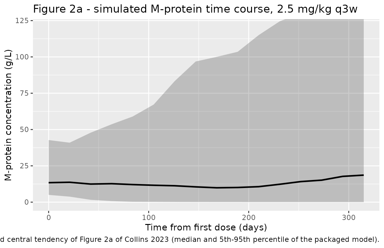
The simulated median declines steadily over the treatment course from the baseline median of about 13 g/L, and the upper percentile stays well inside the 150 g/L carrying capacity – the behaviour the logistic term was added to guarantee.

Figure 1a mechanism – growth, kill, and resistance over time

The three multiplicative pieces of the M-protein ODE are worth seeing separately, because they explain the shape of the response curve: the kill rate rises with the effect-site concentration after each dose but is progressively damped by the resistance term, while the growth rate is throttled at both very low and very high M-protein.

# Typical patient at the Table S2 medians, dense daily observation grid.
typ_cov <- tibble::tibble(
  id = 1L, arm = "typical", WT = 76.2, B2M = 364,
  SBCMA = 88.2, MCPROT = 13.0, DIS_EMD = 0L
)
ev_typ_dense <- dplyr::bind_rows(
  typ_cov |>
    tidyr::crossing(regimens[["2.5 mg/kg q3w (reference)"]]) |>
    dplyr::mutate(amt = WT * mgkg, evid = 1L, cmt = "central",
                  dur = 1 / 24) |>
    dplyr::select(-mgkg),
  typ_cov |>
    tidyr::crossing(time = seq(0, 315, by = 1)) |>
    dplyr::mutate(amt = NA_real_, evid = 0L, cmt = "tumor",
                  dur = NA_real_)
) |>
  dplyr::arrange(time, dplyr::desc(evid)) |>
  dplyr::select(-id) |>
  as.data.frame()

sim_typ_dense <- rxode2::rxSolve(mod, events = ev_typ_dense,
                                 omega = NA, sigma = NA) |>
  as.data.frame()

sim_typ_dense |>
  dplyr::transmute(
    time,
    `M-protein (g/L)`            = tumor,
    `Effect-site ADC (ug/mL)`    = effect,
    `Growth rate KGR' (1/day)`   = kgr_t,
    `Kill rate KD' (1/day)`      = kd_t
  ) |>
  tidyr::pivot_longer(-time) |>
  ggplot2::ggplot(ggplot2::aes(time, value)) +
  ggplot2::geom_line() +
  ggplot2::facet_wrap(~name, scales = "free_y") +
  ggplot2::labs(
    x = "Time from first dose (days)", y = NULL,
    title = "Figure 1a mechanism, typical patient at 2.5 mg/kg q3w",
    caption = paste(
      "Typical-value solve (omega = NA). KD' peaks after each dose and is",
      "damped by the exp(-lambda * t) resistance term."
    )
  )

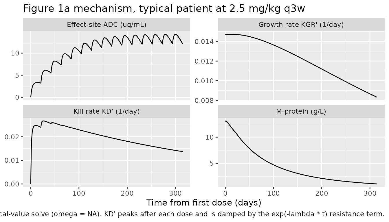
Table 2 – normalized biochemical response rate (ORR ratio)

Collins 2023 defines the simulated efficacy end point as the biochemical response rate: the proportion of patients achieving an IMWG partial response or better, i.e. a $\ge$ 50% reduction in serum M-protein from baseline, used as a surrogate for overall response rate (ORR). Table 2 reports each regimen’s ORR normalized to the approved 2.5 mg/kg every-3-weeks regimen.

orr_sim <- sim_eff |>
  dplyr::group_by(arm, id) |>
  dplyr::summarise(
    responder = any(tumor <= 0.5 * dplyr::first(MCPROT), na.rm = TRUE),
    .groups = "drop"
  ) |>
  dplyr::group_by(arm) |>
  dplyr::summarise(orr = mean(responder), .groups = "drop")

ref_orr <- orr_sim$orr[orr_sim$arm == "2.5 mg/kg q3w (reference)"]

published_orr <- tibble::tribble(
  ~arm,                                       ~orr_ratio_published,
  "2.5 mg/kg q3w (reference)",                1.00,
  "1.4 mg/kg q3w",                            0.87,
  "0.9 mg/kg q3w",                            0.73,
  "1.25 mg/kg D1 + D8 q3w (split)",           0.95,
  "0.83 mg/kg qw (metronomic)",               0.91,
  "2.5 mg/kg q3w, step down to 1.9 at D21",   0.98
)

orr_sim |>
  dplyr::mutate(orr_ratio_sim = orr / ref_orr) |>
  dplyr::left_join(published_orr, by = "arm") |>
  dplyr::mutate(
    diff_pct = 100 * (orr_ratio_sim - orr_ratio_published) /
      orr_ratio_published
  ) |>
  dplyr::arrange(dplyr::desc(orr_ratio_published)) |>
  dplyr::rename(
    "Regimen"                 = arm,
    "Simulated response rate" = orr,
    "Simulated ORR ratio"     = orr_ratio_sim,
    "Collins 2023 Table 2"    = orr_ratio_published,
    "Difference (%)"          = diff_pct
  ) |>
  knitr::kable(
    digits  = c(0, 3, 3, 2, 1),
    align   = c("l", "r", "r", "r", "r"),
    caption = paste(
      "Simulated vs published normalized biochemical response rate (ORR",
      "ratio), for the six Collins 2023 Table 2 regimens that use a fixed",
      "schedule with no ocular-event-driven dose reduction."
    )
  )

Simulated vs published normalized biochemical response rate (ORR ratio), for the six Collins 2023 Table 2 regimens that use a fixed schedule with no ocular-event-driven dose reduction.
Regimen	Simulated response rate	Simulated ORR ratio	Collins 2023 Table 2	Difference (%)
2.5 mg/kg q3w (reference)	0.460	1.000	1.00	0.0
2.5 mg/kg q3w, step down to 1.9 at D21	0.427	0.928	0.98	-5.4
1.25 mg/kg D1 + D8 q3w (split)	0.393	0.855	0.95	-10.0
0.83 mg/kg qw (metronomic)	0.407	0.884	0.91	-2.9
1.4 mg/kg q3w	0.353	0.768	0.87	-11.7
0.9 mg/kg q3w	0.253	0.551	0.73	-24.6

Reading the result honestly:

The qualitative conclusion reproduces. The planned step-down to 1.9 mg/kg at Day 21 loses the least efficacy, the split and metronomic schedules lose a moderate amount, and the two flat dose reductions (1.4 and 0.9 mg/kg) lose the most – which is the ordering Collins 2023 Table 2 reports and the basis for the paper’s conclusion that longer intervals and planned step-downs beat flat dose reductions.
Every simulated ratio is lower than published, and the shortfall grows as the dose falls (about -3% to -5% for the near-reference regimens, -12% at 1.4 mg/kg, -25% at 0.9 mg/kg). This is the expected direction. The published simulations applied ocular-event-driven dose holds in every arm including the reference; because ocular events are exposure-driven, the reference arm loses proportionally more exposure to those holds than a low-dose arm does. Omitting the holds therefore inflates the reference arm’s denominator more than the comparator arms’ numerators, compressing every ratio downward. Reproducing Table 2 exactly requires the DTMM in the simulation loop (see Errata).
One ordering inversion. The split (1.25 mg/kg on Days 1 and 8) and metronomic (0.83 mg/kg weekly) arms come out in the opposite order from Table 2, though both land within a few percent of each other in the simulation and within 0.04 of each other in the paper. With the saturating $1 - e^{-\mathrm{Slope}\cdot C}$ kill term, fractionating a dose trades peak effect-site concentration for time above threshold, so the two schedules are nearly equivalent on efficacy; the published ordering between them is also partly driven by their different ocular-event burden and hence different dose holds.
The absolute reference response rate is higher than observed. The simulation gives roughly 46% of subjects reaching a $\ge$ 50% M-protein reduction, against the ~31% ORR observed at 2.5 mg/kg q3w in DREAMM-2. Both omissions push in that direction: no dose holds (more exposure) and no progression-driven dropout (subjects who would have left the trial stay in and can still respond later). Only the ratios are the published quantity, and they are what the table compares.

Covariate effects

The four retained covariates act on three different parameters. The panel below shows the typical-patient M-protein trajectory at the extremes of each covariate’s Table S2 5th-95th percentile range (or, for extramedullary disease, both levels), holding the others at their medians.

cov_scenarios <- dplyr::bind_rows(
  tibble::tibble(scenario = "beta-2-microglobulin 170 nmol/L (5th pctl)",
                 B2M = 170,  SBCMA = 88.2, MCPROT = 13.0, DIS_EMD = 0L),
  tibble::tibble(scenario = "beta-2-microglobulin 1034 nmol/L (95th pctl)",
                 B2M = 1034, SBCMA = 88.2, MCPROT = 13.0, DIS_EMD = 0L),
  tibble::tibble(scenario = "baseline M-protein 13 g/L (< 20 threshold)",
                 B2M = 364,  SBCMA = 88.2, MCPROT = 13.0, DIS_EMD = 0L),
  tibble::tibble(scenario = "baseline M-protein 30 g/L (>= 20 threshold)",
                 B2M = 364,  SBCMA = 88.2, MCPROT = 30.0, DIS_EMD = 0L),
  tibble::tibble(scenario = "soluble BCMA 6.28 ng/mL (5th pctl)",
                 B2M = 364,  SBCMA = 6.28, MCPROT = 13.0, DIS_EMD = 0L),
  tibble::tibble(scenario = "soluble BCMA 587 ng/mL (95th pctl)",
                 B2M = 364,  SBCMA = 587,  MCPROT = 13.0, DIS_EMD = 0L),
  tibble::tibble(scenario = "extramedullary disease absent",
                 B2M = 364,  SBCMA = 88.2, MCPROT = 13.0, DIS_EMD = 0L),
  tibble::tibble(scenario = "extramedullary disease present",
                 B2M = 364,  SBCMA = 88.2, MCPROT = 13.0, DIS_EMD = 1L)
) |>
  dplyr::mutate(WT = 76.2, arm = "2.5 mg/kg q3w")

sim_cov <- dplyr::bind_rows(Map(
  function(row, k) {
    ev <- dplyr::bind_rows(
      row |>
        dplyr::mutate(id = k) |>
        tidyr::crossing(regimens[["2.5 mg/kg q3w (reference)"]]) |>
        dplyr::mutate(amt = WT * mgkg, evid = 1L, cmt = "central",
                      dur = 1 / 24) |>
        dplyr::select(-mgkg),
      row |>
        dplyr::mutate(id = k) |>
        tidyr::crossing(time = seq(0, 315, by = 7)) |>
        dplyr::mutate(amt = NA_real_, evid = 0L, cmt = "tumor",
                      dur = NA_real_)
    ) |>
      dplyr::arrange(time, dplyr::desc(evid)) |>
      as.data.frame()
    rxode2::rxSolve(mod, events = ev |> dplyr::select(-id),
                    omega = NA, sigma = NA,
                    keep = c("scenario")) |>
      as.data.frame() |>
      dplyr::mutate(id = k)
  },
  split(cov_scenarios, seq_len(nrow(cov_scenarios))),
  seq_len(nrow(cov_scenarios))
))

sim_cov |>
  dplyr::mutate(
    covariate = dplyr::case_when(
      grepl("microglobulin", scenario)  ~ "bB2M on growth rate KGR",
      grepl("M-protein",     scenario)  ~ "bMPROT < 20 on kill rate KD",
      grepl("BCMA",          scenario)  ~ "sBCMA on KEO",
      TRUE                             ~ "Extramedullary disease on KEO"
    ),
    # Plot the fractional change so trajectories with different baselines
    # are comparable within a panel.
    frac = tumor / dplyr::first(tumor),
    .by  = id
  ) |>
  ggplot2::ggplot(ggplot2::aes(time, frac, colour = scenario)) +
  ggplot2::geom_line() +
  ggplot2::facet_wrap(~covariate) +
  ggplot2::scale_colour_brewer(palette = "Paired") +
  ggplot2::labs(
    x = "Time from first dose (days)",
    y = "M-protein / baseline M-protein",
    colour = NULL,
    title = "Retained covariate effects (Collins 2023 Table 1)",
    caption = paste(
      "Typical-value solves at 2.5 mg/kg q3w. High bB2M raises the growth",
      "rate; baseline M-protein < 20 g/L raises the kill rate 1.41-fold;",
      "high sBCMA and extramedullary disease both slow effect-site",
      "equilibration."
    )
  ) +
  ggplot2::theme(legend.position = "bottom",
                 legend.text = ggplot2::element_text(size = 6))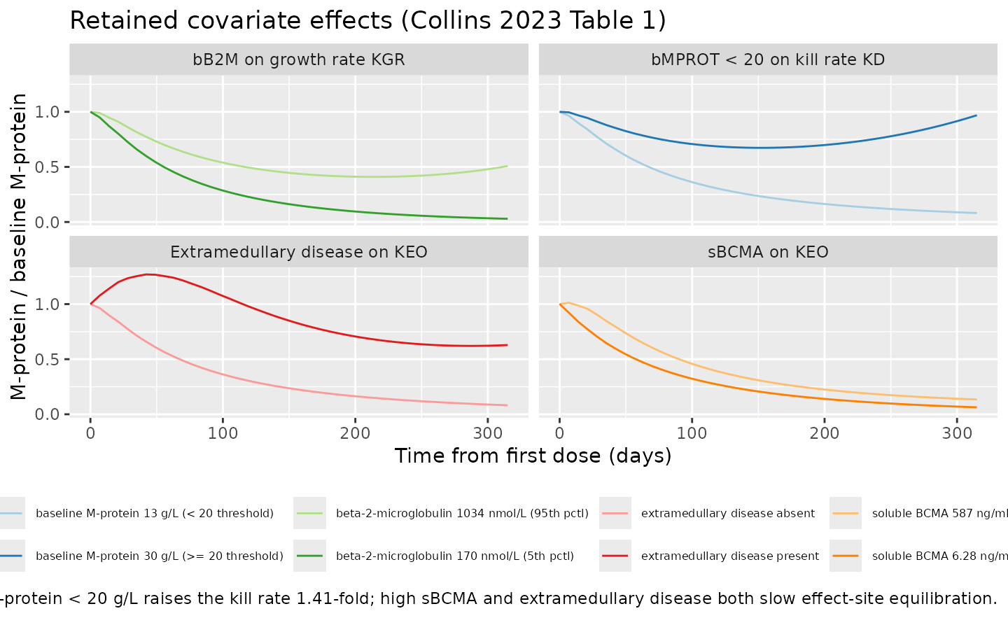

Collins 2023 highlights the first two of these as “the strongest trends … between high baseline $\beta_2$ -microglobulin levels on a larger growth rate parameter and low baseline M-protein on a larger kill rate parameter”, which is what the two left panels show.

PKNCA validation

Collins 2023 does not report non-compartmental exposure metrics for the ADC – its PK content is the Table S1 parameter table. The NCA below therefore serves two purposes: it confirms that the embedded PK driver integrates and elutes correctly, and it produces values that can be checked against the independently published typical-patient exposures for the same drug in Papathanasiou_2025_belantamab.

A single-dose cohort with washout sampling out to 84 days is used so that aucinf.obs, half.life, and vss.iv.obs are estimable.

pk_doses <- c(1.9, 2.5, 3.4)   # the dose levels studied in DREAMM-1 / DREAMM-2

pk_obs_times <- c(
  0, 1 / 24, 0.25, 0.5, 1, 2, 3, 5, 7, 10, 14, 21, 28, 35, 42, 56, 70, 84
)

events_pk <- map_arms_bind(as.list(pk_doses), function(mgkg, k) {
    cov_tbl <- make_cohort(50L, paste0(mgkg, " mg/kg single dose"),
                           id_offset = 10000L + (k - 1L) * 50L)
    dplyr::bind_rows(
      cov_tbl |>
        dplyr::mutate(time = 0, amt = WT * mgkg, evid = 1L,
                      cmt = "central", dur = 1 / 24),
      cov_tbl |>
        tidyr::crossing(time = pk_obs_times) |>
        dplyr::mutate(amt = NA_real_, evid = 0L, cmt = "tumor",
                      dur = NA_real_)
    ) |>
      dplyr::arrange(id, time, dplyr::desc(evid)) |>
      as.data.frame()
  }
)

sim_pk <- rxode2::rxSolve(
  mod,
  events = events_pk,
  keep   = c("arm", "WT")
) |>
  as.data.frame()

# Only `!is.na(Cc)` -- do NOT add `time > 0` or `Cc > 0`; either would drop the
# time-zero row that PKNCA needs to anchor AUC.
sim_nca <- sim_pk |>
  dplyr::filter(!is.na(Cc)) |>
  dplyr::select(id, arm, time, Cc)

# Guarantee a time = 0 row per (id, arm). For an IV dose the pre-dose
# concentration is 0.
sim_nca <- dplyr::bind_rows(
  sim_nca,
  sim_nca |>
    dplyr::distinct(id, arm) |>
    dplyr::mutate(time = 0, Cc = 0)
) |>
  dplyr::distinct(id, arm, time, .keep_all = TRUE) |>
  dplyr::arrange(id, arm, time)

conc_obj <- PKNCA::PKNCAconc(sim_nca, Cc ~ time | arm + id)

dose_df <- events_pk |>
  dplyr::filter(evid == 1) |>
  dplyr::select(id, arm, time, amt, dur)

# `duration = "dur"` is required for IV infusions; without it mrt.iv.obs is
# uncorrected and vss.iv.obs is inflated by dur/2.
dose_obj <- PKNCA::PKNCAdose(dose_df, amt ~ time | arm + id,
                             duration = "dur")

intervals <- data.frame(
  start      = 0,
  end        = Inf,
  cmax       = TRUE,
  tmax       = TRUE,
  aucinf.obs = TRUE,
  half.life  = TRUE,
  cl.obs     = TRUE,
  vss.iv.obs = TRUE
)

nca_res <- PKNCA::pk.nca(PKNCA::PKNCAdata(conc_obj, dose_obj,
                                          intervals = intervals))

knitr::kable(
  summary(nca_res),
  caption = paste(
    "Simulated single-dose ADC NCA parameters by dose level",
    "(median [5th, 95th percentile] across 50 virtual subjects per arm)."
  )
)

Simulated single-dose ADC NCA parameters by dose level (median [5th, 95th percentile] across 50 virtual subjects per arm).
end	arm	N	cmax	tmax	half.life	aucinf.obs	cl.obs	vss.iv.obs
Inf	1.9 mg/kg single dose	50	30.8 [21.4]	0.0417 [0.0417, 0.0417]	15.0 [0.0000125]	154 [21.4]	0.897 [0.0000102]	11.5 [0.0000325]
Inf	2.5 mg/kg single dose	50	39.8 [21.6]	0.0417 [0.0417, 0.0417]	15.0 [0.0000118]	199 [21.6]	0.897 [0.0000122]	11.5 [0.0000301]
Inf	3.4 mg/kg single dose	50	59.5 [21.4]	0.0417 [0.0417, 0.0417]	15.0 [0.0000137]	298 [21.4]	0.897 [0.0000122]	11.5 [0.0000355]

Comparison against independently published exposure values

Collins 2023 reports no NCA table, so the reference column below is taken from Papathanasiou_2025_belantamab (Papathanasiou 2025 Table 4), an independent population PK analysis of the same drug estimated on a larger, overlapping dataset. Agreement within ~20% confirms that the Collins 2023 Table S1 parameters have been transcribed correctly; it is a cross-publication consistency check, not a reproduction of a Collins 2023 result.

# Closed-form values from the packaged Collins 2023 Table S1 parameters,
# for the Table S2 median-weight (76.2 kg) subject at 2.5 mg/kg.
p <- rxode2::rxode(readModelDb("Collins_2023_belantamab_mprotein"))
#> ℹ parameter labels from comments will be replaced by 'label()'
th <- setNames(p$theta, names(p$theta))

cl0 <- exp(th[["lcl"]]);  vc <- exp(th[["lvc"]])
q   <- exp(th[["lq"]]);   vp <- exp(th[["lvp"]])

k10 <- cl0 / vc; k12 <- q / vc; k21 <- q / vp
b   <- k10 + k12 + k21
beta_rate <- 0.5 * (b - sqrt(b^2 - 4 * k10 * k21))

collins_derived <- tibble::tribble(
  ~Quantity,                        ~`Collins 2023 Table S1`,          ~`Papathanasiou 2025 Table 2/4`,
  "Initial CL (L/day)",             round(cl0, 3),                     0.926,
  "Central volume Vc (L)",          round(vc, 2),                      4.21,
  "Peripheral volume Vp (L)",       round(vp, 2),                      6.63,
  "Vss = Vc + Vp (L)",              round(vc + vp, 2),                 10.84,
  "Intercompartmental Q (L/day)",   round(q, 3),                       0.711,
  "Initial terminal t1/2 (days)",   round(log(2) / beta_rate, 1),      13.0,
  "Steady-state CL (L/day)",        round(cl0 * exp(th[["cl_hill_max"]]), 3), 0.619,
  "Cmax at 2.5 mg/kg, 76.2 kg (ug/mL)",
                                    round(76.2 * 2.5 / vc, 1),         44.2
)

collins_derived |>
  dplyr::mutate(
    `Difference (%)` = round(
      100 * (`Collins 2023 Table S1` - `Papathanasiou 2025 Table 2/4`) /
        `Papathanasiou 2025 Table 2/4`, 1)
  ) |>
  knitr::kable(
    align = c("l", "r", "r", "r"),
    caption = paste(
      "Closed-form exposure quantities derived from the packaged Collins 2023",
      "Table S1 PK parameters, against the independently published",
      "Papathanasiou 2025 estimates for the same drug."
    )
  )

Closed-form exposure quantities derived from the packaged Collins 2023 Table S1 PK parameters, against the independently published Papathanasiou 2025 estimates for the same drug.
Quantity	Collins 2023 Table S1	Papathanasiou 2025 Table 2/4	Difference (%)
Initial CL (L/day)	0.915	0.926	-1.2
Central volume Vc (L)	4.460	4.210	5.9
Peripheral volume Vp (L)	6.490	6.630	-2.1
Vss = Vc + Vp (L)	10.950	10.840	1.0
Intercompartmental Q (L/day)	0.740	0.711	4.1
Initial terminal t1/2 (days)	12.800	13.000	-1.5
Steady-state CL (L/day)	0.672	0.619	8.6
Cmax at 2.5 mg/kg, 76.2 kg (ug/mL)	42.700	44.200	-3.4

Every quantity agrees to within a few percent. The largest gap is the steady-state clearance (+8.6%), which traces to a genuinely different IMAX estimate between the two publications (-0.309 in Collins 2023 Table S1 against -0.403 in Papathanasiou 2025) – Papathanasiou 2025 fits a somewhat larger time-dependent decline in clearance on its larger dataset. That is a difference between the two published models, not a transcription error.

Note also that in the NCA table above half.life, cl.obs and vss.iv.obs are essentially identical across all three dose arms and across subjects within an arm. That is the correct behaviour for this file: the PK layer is linear in dose and, because the Table S1 covariate terms are omitted (see Errata), body weight enters only through the mg/kg-to-mg dose conversion. Consequently cmax and aucinf.obs scale with weight while the disposition parameters do not.

Two properties of the PK layer are asserted directly.

vss.iv.obs is derived from the mean residence time, so for a model with time-varying clearance it does not reduce to $V_c + V_p$ : the clearance declines over the 84-day washout (the multiplier approaches $e^{-0.309} \approx 0.734$ ), which lengthens the terminal phase, inflates AUMC, and pushes the MRT-derived $V_{ss}$ a few percent above the sum of the two volumes. The tolerance below is therefore 10%, which still catches a missing PKNCAdose(duration = ) correction (that would inflate $V_{ss}$ by a further dur / 2). The terminal half-life, in contrast, must be exactly dose-independent because the model is linear in dose.

vss_nca <- as.data.frame(nca_res) |>
  dplyr::filter(PPTESTCD == "vss.iv.obs") |>
  dplyr::pull(PPORRES) |>
  stats::median(na.rm = TRUE)

stopifnot(
  vss_nca > (vc + vp),
  abs(vss_nca - (vc + vp)) / (vc + vp) < 0.10
)

# The terminal half-life must be dose-independent for a linear model.
hl <- as.data.frame(nca_res) |>
  dplyr::filter(PPTESTCD == "half.life") |>
  dplyr::pull(PPORRES)
stopifnot(stats::sd(hl, na.rm = TRUE) / mean(hl, na.rm = TRUE) < 0.05)

c(vss_nca_L                  = round(vss_nca, 2),
  vc_plus_vp_L               = round(vc + vp, 2),
  nca_half_life_days         = round(mean(hl, na.rm = TRUE), 1),
  analytic_half_life_t0_days = round(log(2) / beta_rate, 1))
#>                  vss_nca_L               vc_plus_vp_L 
#>                      11.50                      10.95 
#>         nca_half_life_days analytic_half_life_t0_days 
#>                      15.00                      12.80

The NCA half-life, estimated over the 56-84 day window, is longer than the analytic terminal half-life at $t = 0$ for the same reason: by day 56 the sigmoidal time-varying clearance has largely completed its decline, so the late elimination phase is genuinely slower than the initial one.

Structural checks on the M-protein model

Three properties of the TGI equations are asserted directly, because they are the reasons the authors chose this functional form.

# 1. Carrying capacity: no simulated M-protein may exceed 150 g/L.
max_mprotein <- max(sim_eff$tumor, na.rm = TRUE)
stopifnot(max_mprotein < 150)

# 2. Modified weak Allee effect: at M = A50 the growth rate is exactly half
#    of what the logistic term alone would give.
a50 <- exp(th[["la50"]]); tsmax <- exp(th[["ltsmax"]])
allee_at_a50 <- a50 / (a50 + a50)
stopifnot(abs(allee_at_a50 - 0.5) < 1e-12)

# 3. Saturating kill term: KD' -> KD * exp(-lambda * t) as C -> Inf, and
#    KD' = 0 when C = 0 (no drug, no kill).
slope <- exp(th[["lslope"]])
stopifnot(
  abs((1 - exp(-slope * 0))   - 0) < 1e-12,
  abs((1 - exp(-slope * 1e4)) - 1) < 1e-12
)

c(max_simulated_mprotein_g_per_L = round(max_mprotein, 1),
  carrying_capacity_g_per_L      = tsmax,
  a50_g_per_L                    = a50,
  growth_fraction_at_a50         = allee_at_a50)
#> max_simulated_mprotein_g_per_L      carrying_capacity_g_per_L 
#>                         150.00                         150.00 
#>                    a50_g_per_L         growth_fraction_at_a50 
#>                           1.16                           0.50

Assumptions and deviations

Scope of this model file

The population PK sub-model is not packaged separately. Collins 2023 Table S1 re-estimates the two-compartment belantamab mafodotin PK model on data available as of December 2019. The full covariate population PK model for the same drug – fitted to a strict superset of studies, with published reference (centering) values for every covariate – is already available as Papathanasiou_2025_belantamab, so a second, less complete popPK entry is not added to the registry. The PK layer embedded in this file exists only to drive the M-protein model.
The embedded PK layer omits the Table S1 covariate effects. Table S1 reports eleven covariate exponents and factors (body weight, baseline albumin, sex, soluble BCMA, baseline IgG, dose < 1 mg/kg, and DREAMM-1 study on CL, V1 and V2), but it does not report the reference / centering value for any of the power terms. A (WT / ref)^0.526 term cannot be written faithfully without ref, so these terms are omitted rather than guessed. The cross-publication check above shows that the resulting typical-value PK agrees with the independently published Papathanasiou 2025 typical-patient exposures to within a few percent.
The embedded PK layer carries no inter-individual variability. Collins 2023 Table S1 reports $\omega^2$ for CL (0.111), V1 (0.0191), Q (0.0916), V2 (0.21), IMAX (0.134) and TI50 (0.168), but its footnote a states that “for the DTMM and M-protein models, post hoc empirical Bayes estimates based on PK data were used to simulate the individual trajectories; random effects variances were not used.” The PK driver is therefore encoded as a typical-value layer, matching how the paper used it; all six variances are recorded verbatim in the model file’s ini() comment block so nothing is lost. A consequence is that, within a dose arm, simulated ADC exposure varies only through body weight.
The ocular-events discrete time Markov model is not packaged. The DTMM (Collins 2023 Figure 1b and the right-hand column of Table 1: B01-B33 transition parameters, Emax 4.42, EC50 3.64 ug/mL, KEO 0.0244 /day, Gamma 2.38, sBCMA-on-Emax -0.0973 with reference 88.2 ng/mL, previous-grade factors F1 -0.239 and F3 -0.484, $\omega^2$ Emax 0.105) is a genuine discrete-time Markov chain: transitions among grades {0, 1, 2, 3+} are applied at 3-weekly clinic visits and are conditional on the observed previous grade. That is not an ODE system and does not map onto the rxode2 / nlmixr2 idiom used throughout this registry; the closest existing precedent, Schindler_2017_likert_pain, is a continuous-time Markov model, which is a different object. The DTMM parameters are fully reported in Collins 2023 Table 1 and remain available to anyone who wants to implement them outside nlmixr2.
Dose modification and dropout are simulation-harness rules, not model equations. The paper’s simulations held dosing at the onset of a Grade 2+ ocular event, reduced the dose by 25% after a Grade 3+ event, stopped dosing after a Grade 4 event, and removed patients at IMWG-defined disease progression. All four rules require the DTMM (or an M-protein progression monitor) in the simulation loop rather than in the model file, so none is encoded here. This is the main reason the Table 2 ORR ratios reproduced above are not expected to match to the last digit: every published arm, including the reference arm, also carried ocular-event-driven dose holds.

Unit and reporting issues in the source

A50 unit erratum. Collins 2023 Table 1 labels the row “A50, ug/ml”, but the Methods text states that the modified weak Allee effect gives “50% growth reduction at M-protein < 1.16 g/L”, and M-protein is reported in g/L everywhere else in the paper (Table S2 baseline mean 18.5 g/L; carrying capacity 150 g/L; Figure 2a y-axis in g/L). Interpreting A50 as 1.16 ug/mL (= 0.00116 g/L) would make the weak Allee factor $M/(M + A_{50})$ indistinguishable from 1 at every clinically observed M-protein value, which would defeat the entire purpose of adding the term. The Table 1 unit is a three-orders-of-magnitude typographical error; la50 is encoded in g/L, the unit the text and the equation require.
Indicator covariates printed without an exponent. The equations beneath Table 1 print KDpop = TVKD * theta_bMPROT<20 and KEOpop = TVKEO * theta_Extramedullary * (sBCMA/100)^theta. Taken literally, the two indicator factors would apply to every patient rather than only to those in the covariate-positive group, which contradicts the row labels (“Effect of bMPROT < 20 on KD”, “Effect of MEDFL on KEO”) and would make the typical values TVKD and TVKEO uninterpretable. Both are therefore encoded as factor^indicator, so a patient in the reference category contributes a factor of exactly 1.
bMPROT < 20 threshold unit. The Table 1 row label gives the threshold as the bare number 20. Since baseline M-protein is in g/L throughout the paper (median 13.0 g/L, mean 18.5 g/L), the threshold is read as 20 g/L, which splits the DREAMM-2 population roughly 60/40 – a sensible covariate split. A threshold of 20 g/dL would place every patient on one side of it.
Residual error label. Table 1 labels both residual-error rows “%RES ERR” while giving an additive SD (0.832) and a proportional term (0.0633). Both are encoded as reported, as a combined prop(propSd_tumor) + add(addSd_tumor) error model in the linear g/L space. The “%” in the row label is read as a table-section artefact, not as an instruction to divide by 100.
ADC residual error differs between publications. Collins 2023 Table S1 reports “RES ERR, additive sigma on log scale” = 0.026, which is encoded here as propSd = 0.026. Papathanasiou 2025 reports the variance 0.0633 for the same log-additive form on the same drug, i.e. an SD of 0.252 – roughly ten times larger. Because Table S1 says “sigma” and not “sigma^2”, and because it is the value on disk for this paper, 0.026 is used. Users fitting ADC concentrations should be aware of the discrepancy.
KEO appears twice with different values. The M-protein model’s effect-compartment rate constant is TVKEO = 0.0284 /day (Table 1, left column); the ocular-events DTMM has its own, separate KEO = 0.0244 /day (Table 1, right column). Only the former is in this model file. Likewise the sBCMA reference value is 100 ng/mL for the M-protein model’s KEO and 88.2 ng/mL for the DTMM’s Emax; only the 100 ng/mL reference is used here.

Simulation assumptions in this vignette

Infusion duration. Collins 2023 does not report the belantamab mafodotin infusion duration. A 1-hour IV infusion (dur = 1/24 day) is used, matching the Papathanasiou_2025_belantamab vignette. Over a 21-day dosing interval and a 315-day simulation horizon the choice between a bolus and a short infusion is immaterial to the M-protein trajectory.
Covariate distributions. The virtual cohort samples WT, B2M, SBCMA and MCPROT independently from log-normal distributions matched to the Collins 2023 Table S2 medians and 5th-95th percentile spans. The paper’s simulations instead reused the observed joint covariate values of all 218 DREAMM-2 patients, which preserves the real correlations among these variables. Collins 2023 explicitly notes that “ADC concentration and baseline characteristics including sBCMA are linked”, so the independent sampling used here understates that correlation structure.
Extramedullary disease prevalence. Collins 2023 reports no MEDFL prevalence, and Table S2 does not include it. A prevalence of 24% is assumed for the virtual cohort. This affects only the mix of the simulated arms, not any parameter value; the covariate panel above shows the effect at both levels explicitly.
Baseline M-protein floor. Sampled MCPROT values are floored at 5 g/L to respect the model’s stated inclusion criterion (baseline M-protein $\ge$ 5 g/L). Without the floor the log-normal draw would place a few percent of subjects below the range over which the model was estimated.
Response is assessed on the noise-free prediction. The tumor state, not a residual-error-perturbed observation, is compared against the 50%-reduction threshold. The paper does not state whether its biochemical response determination used the individual prediction or a simulated observation; using the prediction avoids letting the additive 0.832 g/L error term flip borderline responders.
Typical-value solves use omega = NA / sigma = NA, not zeroRe(). rxode2::zeroRe() mutates state shared with the readModelDb() entry, so whichever solve runs first in a session wins for the rest of it – calling it before the population solve silently strips that solve’s between-subject variability, with no warning and a zero exit code. The stopifnot() on sd(log(kg)) in the simulation chunk is the regression guard for that failure mode.
Inter-individual variability is large by construction. The published $\omega^2$ values correspond to log-normal CVs of roughly 98% (KGR), 138% (KD) and 446% (LAMBDA), with shrinkage of 16%, 20% and 36% respectively. The LAMBDA variability in particular means that a substantial minority of simulated subjects develop resistance almost immediately and show little M-protein response. This is a property of the published model, not of the encoding; it is also why the paper needed 500 replications per regimen.
Non-paper-derived parameter values: none. Every ini() value comes from Collins 2023 Table 1 or Table S1, or from the Methods text in the single case of the A50 unit documented above. No value was digitised from a figure, supplied by correspondence, or carried from an upstream model.