Nebulized and intravenous polymyxin B in plasma and ELF (Li 2025)
Source:vignettes/articles/Li_2025_polymyxinB.Rmd
Li_2025_polymyxinB.RmdModel and source
- Citation: Li X, Zhou L, Wang D, Wu Q, Huang X, Zhang H, Wu W, Liu M, Wu X, Qiu H, Cheng Y. Population pharmacokinetics study on nebulized and intravenous administration of polymyxin B in patients with pneumonia caused by multidrug-resistant gram-negative bacteria. Antimicrob Agents Chemother. 2025;69(5):e00044-25. doi:10.1128/aac.00044-25. PMID 40237505. PMCID PMC12057357.
- Description: Coupled plasma + epithelial-lining-fluid (ELF) population PK model for polymyxin B given intravenously and/or by nebulization to critically ill adults with multidrug-resistant Gram-negative pneumonia (Li 2025). Two two-compartment models with linear elimination: an IV infusion enters the plasma central compartment (central <-> peripheral1, clearance from central), a nebulized dose enters the ELF central compartment (elf <-> lung, clearance from elf) with a fraction F = 0.557 reaching the lung, and the two central compartments exchange through a single inter-compartmental clearance Q = 0.03 L/h. Age is a power covariate on the ELF central volume and serum albumin a power covariate on the ELF clearance, both normalised to the cohort medians (66 years, 32.1 g/L). Exponential IIV on the plasma and ELF central clearances and volumes; one proportional residual error (43%) estimated jointly for the plasma and ELF concentrations. Fit in NONMEM 7.5 (FOCE-I).
- Article: Antimicrob Agents Chemother. 2025;69(5):e00044-25 (open access, PMC12057357)
Population
Li 2025 is a prospective single-centre study (Fujian Medical University Union Hospital, China, January 2022 - October 2024) of 76 critically ill, mechanically ventilated adults with pneumonia caused by microbiologically proven multidrug-resistant Gram-negative bacteria. Every patient received nebulized polymyxin B (25 mg in 5 mL every 12 h over 15 min by vibrating-mesh or jet nebulizer), either alone or together with intravenous polymyxin B (loading dose 100-150 mg, then 40-75 mg every 12 h as ~1 h infusions). Table 1 gives 59 men and 17 women (22.4% female), median age 66.0 years (IQR 55.0-76.3), weight 65.0 kg (54.38-70.0), serum albumin 32.1 g/L (28.5-37.5), Cockcroft-Gault creatinine clearance 55.7 mL/min (35.4-101.3), APACHE II 21 and SOFA 7; 55.3% had sepsis. Patients on continuous renal replacement therapy were excluded.
At steady state (after at least four doses) 156 epithelial lining fluid (ELF) concentrations were obtained from all 76 patients by bronchoalveolar lavage, corrected for dilution with the plasma/BAL urea ratio (Eq. 1), and 188 plasma concentrations from 65 patients, pre-dose and 1, 2, 4, 6, 8 and 12 h after administration. Polymyxin B1 and B2 were summed. The model was fit in NONMEM 7.5 with FOCE-I.
The same information is available programmatically via
readModelDb("Li_2025_polymyxinB")()$population.
Model structure
Figure 2 of the paper couples two two-compartment models. Compartment
1 is the plasma central compartment (IV infusion, clearance CL1),
compartment 2 the plasma peripheral compartment (inter-compartmental
clearance CL2), compartment 3 the ELF central compartment (nebulized
dose, clearance CL3) and compartment 4 the ELF peripheral compartment
(inter-compartmental clearance CL4). The two central compartments
exchange through a single clearance Q, and only a fraction F of a
nebulized dose reaches the ELF. In the package the four states are
central, peripheral1, elf and
lung; following the interpretation the authors cite (Lin et
al.), the ELF peripheral compartment is the deeper lung region the drug
reaches from the airway lining fluid.
Source trace
The per-parameter origin is recorded as an in-file comment next to
each ini() entry in
inst/modeldb/specificDrugs/Li_2025_polymyxinB.R.
| Equation / parameter | Value | Source location |
|---|---|---|
lcl (CL1) |
1.39 L/h | Table 2 (RSE 6%) |
lvc (V1) |
27.6 L | Table 2 (RSE 12%) |
lq (CL2) |
13.11 L/h | Table 2 (RSE 18%) |
lvp (V2) |
17.1 L | Table 2 (RSE 11%) |
lcl_elf (CL3) |
0.186 L/h | Table 2 (RSE 21%) |
lv_elf (V3) |
0.896 L | Table 2 (RSE 19%) |
lq_elf_lung (CL4) |
3.44 L/h | Table 2 (RSE 14%) |
lv_lung (V4) |
4.35 L | Table 2 (RSE 10%) |
lq_elf (Q) |
0.03 L/h | Table 2 (RSE 10%) |
lf_elf (F) |
0.557 | Table 2 (RSE 21%) |
e_age_v_elf |
1.28 | Table 2, “AGE on V3” (RSE 23%); Table S1 model 4 |
e_alb_cl_elf |
-0.893 | Table 2, “ALB on CL3” (RSE 17%); Table S1 model 5 |
etalcl, etalvc
|
0.56, 0.31 | Table 2, omega2 CL1 and V1 (variances) |
etalcl_elf, etalv_elf
|
0.45, 0.53 | Table 2, omega2 CL3 and V3 (variances) |
propSd, propSd_Celf
|
0.43 | Table 2, “Proportional error” (one estimate for both matrices) |
| Covariate reference values | 66 years, 32.1 g/L | Table 1 medians (normalising values not printed; see Assumptions) |
| ODE system | n/a | Figure 2 and its legend (micro-constants k10 … k43) |
f(elf) |
n/a | Discussion: F is “the fraction of drug reaching the lungs” |
Virtual cohort
The observed data are not public. The virtual patients draw age and albumin from normal distributions matching the Table 1 medians and interquartile ranges (truncated to 18-95 years and 15-50 g/L). The random effects are drawn in base R from the model’s OMEGA matrix and passed to the solver as data columns, so the same cohort is produced on every machine and every regimen below is simulated on identical patients.
set.seed(20250517)
mod <- readModelDb("Li_2025_polymyxinB")
ui <- rxode2::rxode2(mod)
#> ℹ parameter labels from comments will be replaced by 'label()'
omega <- ui$omega
n_per_arm <- 200L

draw_etas <- function(n) {
  eta <- matrix(rnorm(n * nrow(omega)), n) %*% chol(omega)
  colnames(eta) <- rownames(omega)
  as.data.frame(eta)
}
rtrunc_norm <- function(n, mean, sd, lower, upper) {
  pmin(pmax(rnorm(n, mean, sd), lower), upper)
}

# IQR / 1.349 is the SD of a normal distribution with that IQR.
patients <- tibble(
  k = seq_len(n_per_arm),
  AGE = rtrunc_norm(n_per_arm, 66, (76.3 - 55.0) / 1.349, 18, 95),
  ALB = rtrunc_norm(n_per_arm, 32.1, (37.5 - 28.5) / 1.349, 15, 50)
) |>
  bind_cols(draw_etas(n_per_arm))

# Dosing every 12 h from time 0 to 84 h (eight doses), so 72-96 h is day 4,
# the interval the paper calls steady state. IV infusions run 1 h with a
# loading dose of twice the maintenance dose; nebulizations run 15 min.
make_events <- function(pat, iv_md, neb_dose, obs_times, id_offset = 0L, arm = "",
                        dose_times = seq(0, 84, by = 12)) {
  pat <- pat |> mutate(id = id_offset + row_number())
  iv <- if (iv_md > 0) {
    tidyr::expand_grid(id = pat$id, time = dose_times) |>
      mutate(amt = ifelse(time == 0, 2 * iv_md, iv_md), cmt = "central", dur = 1)
  }
  neb <- if (neb_dose > 0) {
    tidyr::expand_grid(id = pat$id, time = dose_times) |>
      mutate(amt = neb_dose, cmt = "elf", dur = 0.25)
  }
  doses <- bind_rows(iv, neb) |> mutate(evid = 1L, dvid = NA_integer_)
  obs <- tidyr::expand_grid(id = pat$id, time = obs_times) |>
    mutate(amt = 0, cmt = "central", dur = 0, evid = 0L, dvid = 1L)
  bind_rows(doses, obs) |>
    left_join(pat |> select(-k), by = "id") |>
    mutate(arm = arm) |>
    arrange(id, time, desc(evid))
}

solve_events <- function(events) {
  # Random effects come from the data columns; omega/sigma = NA stops the
  # solver from drawing its own (multi-endpoint model).
  rxode2::rxSolve(
    mod, events = events, omega = NA, sigma = NA, useLinCmt = FALSE,
    keep = "arm", returnType = "data.frame"
  )
}
Concentration-time profiles at steady state
Figure 1 of the paper shows the observed ELF (A) and plasma (B) concentrations against time after dose at steady state. The study regimen was 25 mg nebulized every 12 h, with or without IV polymyxin B; the median daily IV dose of 1.82 mg/kg at the median weight of 65 kg is about 60 mg every 12 h.
obs_grid <- seq(72, 96, by = 0.25)
ev_fig1 <- bind_rows(
  make_events(patients, iv_md = 60, neb_dose = 25, obs_times = obs_grid,
              id_offset = 0L, arm = "Nebulized 25 mg + IV 60 mg q12h"),
  make_events(patients, iv_md = 0, neb_dose = 25, obs_times = obs_grid,
              id_offset = 1000L, arm = "Nebulized 25 mg q12h alone")
)
stopifnot(!anyDuplicated(ev_fig1[ev_fig1$evid == 0, c("id", "time")]))
sim_fig1 <- solve_events(ev_fig1)
#> ℹ parameter labels from comments will be replaced by 'label()'
sim_fig1 |>
  filter(time >= 84) |>
  mutate(tad = time - 84) |>
  pivot_longer(c(Celf, Cc), names_to = "matrix", values_to = "conc") |>
  mutate(matrix = ifelse(matrix == "Celf", "(A) ELF", "(B) Plasma")) |>
  group_by(arm, matrix, tad) |>
  summarise(
    Q05 = quantile(conc, 0.05), Q50 = median(conc), Q95 = quantile(conc, 0.95),
    .groups = "drop"
  ) |>
  ggplot(aes(tad, Q50, colour = arm, fill = arm)) +
  geom_ribbon(aes(ymin = Q05, ymax = Q95), alpha = 0.15, colour = NA) +
  geom_line() +
  facet_wrap(~matrix, scales = "free_y") +
  scale_y_log10() +
  labs(
    x = "Time after dose (h)", y = "Polymyxin B (mg/L)", colour = NULL, fill = NULL,
    caption = "Median and 90% interval of model predictions (no residual error). Compare Figure 1 of Li 2025."
  ) +
  theme(legend.position = "bottom")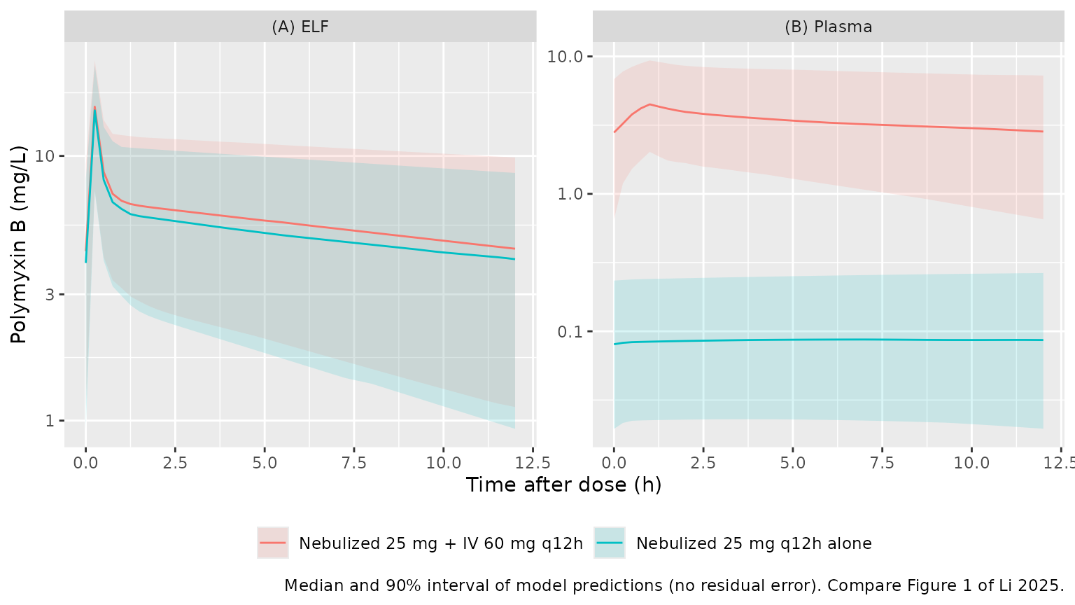
The observed plasma concentrations in Figure 1B lie mostly between 0.5 and 5 mg/L, with the lowest values from patients who received nebulization only, and the simulated plasma bands cover that range. In ELF (Figure 1A) the simulated median of roughly 4-7 mg/L through the middle of the interval matches the observed smooth, but two features of the observed data are outside the simulated 90% band: the early peaks of 20-100 mg/L in the first hour after nebulization, and the fall to below 1 mg/L in many pre-dose samples. The model’s typical ELF peak is about 14 mg/L, because the 15-min nebulization delivers F = 0.557 of the 25 mg dose into a 0.9 L central volume, and the large ELF peripheral compartment (V4 = 4.35 L, CL4 = 3.44 L/h) keeps refilling the central compartment late in the interval. The bands exclude the 43% proportional residual error, which widens them for comparison with observations.
PKNCA validation
PKNCA computes the day-4 (72-96 h) AUC and Cmax in each matrix. Table 1 of the paper reports a cohort median AUC24h of 52.5 mg h/L in ELF and 35.0 mg h/L in plasma, which are compared with the arm closest to the median regimen.
nca_conc <- sim_fig1 |>
  filter(!is.na(Cc)) |>
  select(id, time, arm, Cc, Celf) |>
  pivot_longer(c(Cc, Celf), names_to = "matrix", values_to = "conc") |>
  mutate(matrix = ifelse(matrix == "Celf", "ELF", "Plasma"))

# One dose row per time per subject (amounts summed across routes) so that
# PKNCA sees unique dose times within each group.
nca_dose <- ev_fig1 |>
  filter(evid == 1) |>
  group_by(id, arm, time) |>
  summarise(amt = sum(amt), .groups = "drop") |>
  tidyr::expand_grid(matrix = c("ELF", "Plasma"))

conc_obj <- PKNCA::PKNCAconc(nca_conc, conc ~ time | arm + matrix + id)
dose_obj <- PKNCA::PKNCAdose(nca_dose, amt ~ time | arm + matrix + id)
intervals <- data.frame(start = 72, end = 96, auclast = TRUE, cmax = TRUE)
nca_res <- PKNCA::pk.nca(PKNCA::PKNCAdata(conc_obj, dose_obj, intervals = intervals))

nca_summary <- as.data.frame(nca_res$result) |>
  group_by(arm, matrix, PPTESTCD) |>
  summarise(median = median(PPORRES), .groups = "drop") |>
  pivot_wider(names_from = PPTESTCD, values_from = median)
nca_summary |>
  dplyr::rename(
    "Regimen" = arm, "Matrix" = matrix,
    "Median AUC 72-96 h (mg h/L)" = auclast, "Median Cmax (mg/L)" = cmax
  ) |>
knitr::kable(digits = 1, caption = "Simulated day-4 exposure (PKNCA).")| Regimen | Matrix | Median AUC 72-96 h (mg h/L) | Median Cmax (mg/L) |
|---|---|---|---|
| Nebulized 25 mg + IV 60 mg q12h | ELF | 136.5 | 15.3 |
| Nebulized 25 mg + IV 60 mg q12h | Plasma | 79.5 | 4.5 |
| Nebulized 25 mg q12h alone | ELF | 123.0 | 14.9 |
| Nebulized 25 mg q12h alone | Plasma | 2.0 | 0.1 |
published <- tibble::tribble(
  ~arm,                               ~matrix,  ~auclast,
  "Nebulized 25 mg + IV 60 mg q12h",  "ELF",    52.5,
  "Nebulized 25 mg + IV 60 mg q12h",  "Plasma", 35.0
)
cmp <- nlmixr2lib::ncaComparisonTable(
  simulated = nca_res,
  reference = published,
  by = c("arm", "matrix"),
  units = c(auclast = "mg*h/L"),
  tolerance_pct = 20
)
knitr::kable(cmp, caption = "Simulated day-4 AUC vs Table 1 AUC24h. * differs from reference by >20%.")| NCA parameter | arm | matrix | Reference | Simulated | % diff |
|---|---|---|---|---|---|
| AUClast (mg*h/L) | Nebulized 25 mg + IV 60 mg q12h | ELF | 52.5 | 136 | +159.9%* |
| AUClast (mg*h/L) | Nebulized 25 mg + IV 60 mg q12h | Plasma | 35 | 79.5 | +127.2%* |
Both rows are starred: the simulated AUC over 24 h at the median regimen is roughly two to three times the Table 1 medians. The paper does not say how the Table 1 AUCs were obtained or over which interval, and they are not consistent with the paper’s own target-attainment simulations either (next section), which assume ELF exposures at least as high as this model predicts. Half of the simulated daily AUC, i.e. the AUC over one 12-h dosing interval, is within about 30% of the Table 1 numbers (see also the closed-form check below), so the Table 1 column may hold dosing-interval AUCs. This is recorded as a known discrepancy and was not tuned.
Closed-form steady-state check
For a linear model the steady-state AUC follows from mass balance.
Over one day, with daily nebulized dose Dneb and IV dose
Div, the ELF and plasma AUCs satisfy
F*Dneb + Q*AUCp = (CL3 + Q)*AUCelf and
Div + Q*AUCelf = (CL1 + Q)*AUCp. The typical-value
simulation over day 20 must reproduce the solution of these two
equations.
typical <- patients[1, ] |>
  mutate(AGE = 66, ALB = 32.1, across(starts_with("eta"), ~0))
ev_ss <- make_events(
  typical, iv_md = 60, neb_dose = 25, obs_times = seq(456, 480, by = 0.05),
  dose_times = seq(0, 468, by = 12)
)
sim_ss <- solve_events(ev_ss)
trap <- function(t, y) sum(diff(t) * (head(y, -1) + tail(y, -1)) / 2)
auc_sim <- c(elf = trap(sim_ss$time, sim_ss$Celf), plasma = trap(sim_ss$time, sim_ss$Cc))

p <- ui$theta
cl1 <- exp(p[["lcl"]]); cl3 <- exp(p[["lcl_elf"]]); q <- exp(p[["lq_elf"]]); f <- exp(p[["lf_elf"]])
d_neb <- 50; d_iv <- 120
auc_elf <- (f * d_neb + q * d_iv / (cl1 + q)) / ((cl3 + q) - q^2 / (cl1 + q))
auc_p <- (d_iv + q * auc_elf) / (cl1 + q)
auc_cf <- c(elf = auc_elf, plasma = auc_p)
# Nebulized contribution alone (Div = 0), used in the PTA discussion below.
auc_elf_neb25 <- f * d_neb / ((cl3 + q) - q^2 / (cl1 + q))
knitr::kable(
  data.frame(matrix = names(auc_cf), closed_form = auc_cf, simulated = auc_sim,
             pct_diff = 100 * (auc_sim - auc_cf) / auc_cf),
  digits = 2, row.names = FALSE,
  caption = "Typical-value AUC over one day at steady state (mg h/L)."
)| matrix | closed_form | simulated | pct_diff |
|---|---|---|---|
| elf | 141.09 | 141.09 | 0 |
| plasma | 87.49 | 87.49 | 0 |
# Same parameters on both sides: the gap is numerical (trapezoid on a 0.05 h
# grid, residual approach to steady state at day 20), well under 1%.
stopifnot(all(abs(auc_sim - auc_cf) / auc_cf < 0.01))
Half of these daily values (about 71 mg h/L in ELF and 44 mg h/L in plasma per 12-h interval) is close to the Table 1 AUC24h medians.
Probability of target attainment
The paper’s Monte Carlo simulations (Figures 4-6 and S2-S3) evaluate the day-4 AUC against these targets: plasma AUC/MIC >= 50 (fAUC/MIC 20 with an unbound fraction of 0.42) with AUC > 100 mg h/L as the nephrotoxicity threshold, and ELF AUC/MIC of 326-989 for A. baumannii, 525-527 for K. pneumoniae and 1,326-1,506 for P. aeruginosa. The regimens were IV 50-150 mg q12h (loading dose twice the maintenance dose) and nebulized 25-100 mg q12h, alone or combined.
Because the model is linear, each patient’s day-4 AUC is a sum of an IV part proportional to the IV maintenance dose and a nebulized part proportional to the nebulized dose. Each patient is therefore solved once per route at a unit dose and every regimen in the grid is formed by scaling and adding. The three age and three albumin strata of the paper are represented by one age and one albumin value each.
strata <- tidyr::expand_grid(
  age_group = c("18-40", "40-65", ">65"),
  alb_group = c("<25", "25-35", ">35")
) |>
  mutate(
    AGE = c("18-40" = 30, "40-65" = 52, ">65" = 75)[age_group],
    ALB = c("<25" = 22, "25-35" = 30, ">35" = 40)[alb_group],
    stratum = row_number()
  )
pta_grid_obs <- seq(72, 96, by = 0.1)
unit_auc <- function(route) {
  ev <- bind_rows(lapply(seq_len(nrow(strata)), function(i) {
    pat <- patients |> mutate(AGE = strata$AGE[i], ALB = strata$ALB[i])
    make_events(
      pat,
      iv_md = if (route == "iv") 1 else 0,
      neb_dose = if (route == "neb") 1 else 0,
      obs_times = pta_grid_obs, id_offset = (i - 1L) * 1000L,
      arm = as.character(i)
    )
  }))
  solve_events(ev) |>
    group_by(id, arm) |>
    summarise(elf = trap(time, Celf), plasma = trap(time, Cc), .groups = "drop") |>
    mutate(stratum = as.integer(arm), k = id - (stratum - 1L) * 1000L) |>
    select(stratum, k, elf, plasma)
}
auc_unit <- inner_join(
  unit_auc("iv") |> rename(elf_iv = elf, plasma_iv = plasma),
  unit_auc("neb") |> rename(elf_neb = elf, plasma_neb = plasma),
  by = c("stratum", "k")
) |>
  left_join(strata, by = "stratum")

regimens <- tidyr::expand_grid(iv = c(0, 50, 75, 100, 125, 150), neb = c(0, 25, 50, 75, 100)) |>
  filter(iv + neb > 0)
auc_reg <- tidyr::expand_grid(auc_unit, regimens) |>
  mutate(
    auc_elf = iv * elf_iv + neb * elf_neb,
    auc_plasma = iv * plasma_iv + neb * plasma_neb
  )
Plasma (IV alone)
mics <- c(0.125, 0.25, 0.5, 1, 2, 4)
pta_plasma <- auc_reg |>
  filter(neb == 0) |>
  tidyr::expand_grid(mic = mics) |>
  group_by(iv, mic) |>
  summarise(pta = 100 * mean(auc_plasma / mic >= 50), .groups = "drop")
pta_plasma |>
  mutate(mic = paste0("MIC ", mic)) |>
  pivot_wider(names_from = mic, values_from = pta) |>
  dplyr::rename("IV maintenance dose (mg q12h)" = iv) |>
knitr::kable(digits = 0, caption = "Day-4 plasma PTA (%), AUC/MIC >= 50, all strata pooled (compare Figure S2B).")| IV maintenance dose (mg q12h) | MIC 0.125 | MIC 0.25 | MIC 0.5 | MIC 1 | MIC 2 | MIC 4 |
|---|---|---|---|---|---|---|
| 50 | 100 | 99 | 92 | 65 | 26 | 0 |
| 75 | 100 | 100 | 98 | 80 | 48 | 11 |
| 100 | 100 | 100 | 99 | 92 | 65 | 26 |
| 125 | 100 | 100 | 100 | 96 | 72 | 39 |
| 150 | 100 | 100 | 100 | 98 | 80 | 48 |
tox <- auc_reg |>
  filter(neb == 0) |>
  group_by(iv) |>
  summarise(pct_auc_over_100 = 100 * mean(auc_plasma > 100), .groups = "drop")
tox |>
  dplyr::rename("IV maintenance dose (mg q12h)" = iv, "Day-4 AUC > 100 mg h/L (%)" = pct_auc_over_100) |>
knitr::kable(digits = 0, caption = "Predicted toxicity-threshold exceedance (compare Figure S3).")| IV maintenance dose (mg q12h) | Day-4 AUC > 100 mg h/L (%) |
|---|---|
| 50 | 26 |
| 75 | 48 |
| 100 | 65 |
| 125 | 72 |
| 150 | 80 |
The paper reports that IV 50 and 75 mg q12h reach a plasma PTA of at least 90% for MICs up to 0.5 and 1 mg/L, respectively. The model reproduces the first statement (about 92%) and gives about 80% for the second. The model’s predicted exceedance of the AUC > 100 mg h/L threshold rises more gradually with dose than Figure S3 (25-30% at 75 mg and over 70% at 100 mg q12h): the published curves imply a much narrower spread of AUC than the plasma clearance variance in Table 2 (omega2 = 0.56, a standard deviation of 0.75 on the log scale) generates. The paper simulated “on the original data set”, which may mean the patients’ own parameter estimates rather than fresh draws from the population distribution; the model here uses the published population distribution.
pta_at <- function(d, iv_dose, mic_value) d$pta[d$iv == iv_dose & d$mic == mic_value]
stopifnot(
  # "MICs of <= 0.5 ... IV doses of 50 ... mg q12h" reached PTA >= 90%.
  pta_at(pta_plasma, 50, 0.5) >= 85,
  # The paper reports >= 90%; this model gives about 80% on the fixed base-R
  # cohort, so the bound checks the level without claiming the 90%.
  pta_at(pta_plasma, 75, 1) >= 70
)
ELF
targets <- tibble::tribble(
  ~pathogen,        ~target_low, ~target_high,
  "A. baumannii",   326,         989,
  "K. pneumoniae",  525,         527,
  "P. aeruginosa",  1326,        1506
)
pta_elf <- auc_reg |>
  tidyr::expand_grid(targets) |>
  tidyr::expand_grid(mic = mics) |>
  group_by(pathogen, iv, neb, mic) |>
  summarise(
    pta_low_target = 100 * mean(auc_elf / mic >= first(target_low)),
    pta_high_target = 100 * mean(auc_elf / mic >= first(target_high)),
    .groups = "drop"
  )

# Highest MIC with PTA >= 90%, for IV 0-75 mg q12h combined with each nebulized dose.
pta_elf |>
  filter(iv <= 75, neb > 0) |>
  group_by(pathogen, neb, mic) |>
  summarise(min_pta = min(pta_low_target), .groups = "drop") |>
  group_by(pathogen, neb) |>
  summarise(
    max_mic = if (any(min_pta >= 90)) max(mic[min_pta >= 90]) else NA_real_,
    .groups = "drop"
  ) |>
  pivot_wider(names_from = neb, values_from = max_mic, names_prefix = "Neb ") |>
  dplyr::rename("Pathogen" = pathogen) |>
knitr::kable(caption = "Highest MIC (mg/L) with day-4 ELF PTA >= 90% for every IV dose from 0 to 75 mg q12h, using the lowest target of each range.")| Pathogen | Neb 25 | Neb 50 | Neb 75 | Neb 100 |
|---|---|---|---|---|
| A. baumannii | 0.125 | 0.250 | 0.500 | 0.500 |
| K. pneumoniae | NA | 0.125 | 0.250 | 0.250 |
| P. aeruginosa | NA | NA | 0.125 | 0.125 |
pta_elf |>
  filter(neb %in% c(25, 50, 75, 100), iv %in% c(0, 75, 150)) |>
  arrange(neb, iv) |>
  mutate(regimen = paste0("Neb ", neb, " + IV ", iv), regimen = factor(regimen, levels = unique(regimen))) |>
  ggplot(aes(factor(mic), regimen, fill = pta_low_target)) +
  geom_tile() +
  facet_wrap(~pathogen) +
  scale_fill_gradient(low = "grey85", high = "navy", limits = c(0, 100)) +
  labs(
    x = "MIC (mg/L)", y = "Regimen (mg q12h)", fill = "PTA (%)",
    caption = "Day-4 ELF PTA, lowest target of each range, strata pooled. Compare Figures 4-6 of Li 2025."
  )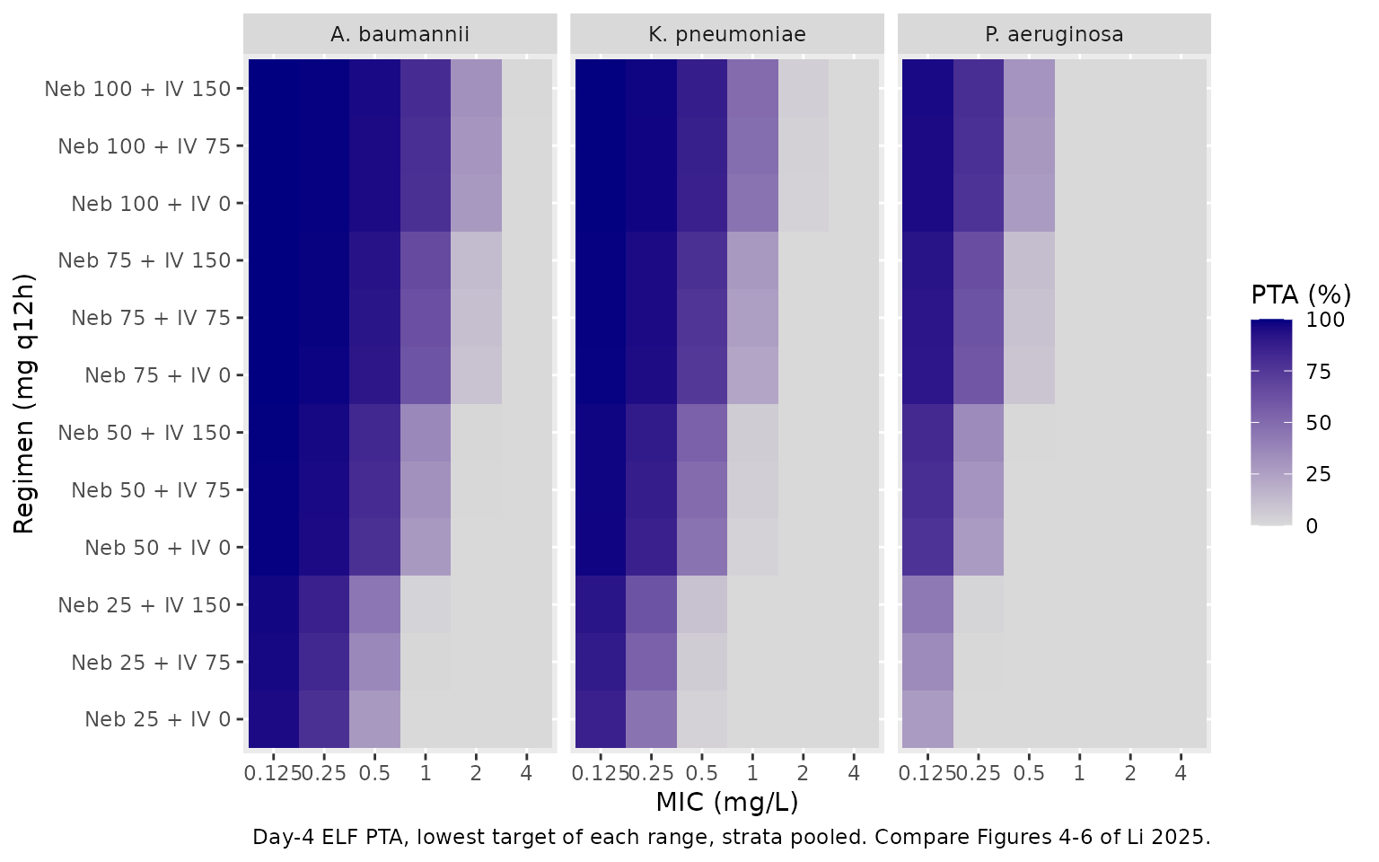
The paper’s ELF conclusions are that IV administration alone (50-150 mg q12h) never reaches the ELF targets, that K. pneumoniae and A. baumannii with MICs of 0.25, 0.5 and 1 mg/L need nebulized doses of at least 25, 50 and 75 mg q12h, and that P. aeruginosa needs higher nebulized doses than the other two. The first conclusion holds in the model, and the last follows directly from the higher P. aeruginosa targets. For the dose-MIC pairs, the model reaches PTA >= 90% one to two MIC dilutions lower than the paper: its typical day-4 ELF AUC for 25 mg q12h nebulized is about 129 mg h/L (from nebulization alone), so a 90% attainment of an AUC/MIC of 525 at MIC 0.25 mg/L would need a narrower spread than the omega2 of 0.45 on CL3 allows. The same narrow spread is visible in the published heat maps, where PTA falls from near 100% to near 0% within one MIC dilution; as for plasma, this points to simulations based on the study patients’ own estimates.
# Paper: "IV administration of 50-150 mg alone failed to achieve the PK/PD
# target values for the three bacteria in ELF", i.e. PTA < 90% everywhere. The
# most favourable IV-only case here (150 mg q12h, A. baumannii at MIC
# 0.125 mg/L against the lowest target of 326) reaches about 23%, because the
# plasma-to-ELF clearance Q (0.03 L/h) is small next to the ELF clearance.
stopifnot(max(pta_elf$pta_low_target[pta_elf$neb == 0]) < 50)
Assumptions and deviations
-
Covariate equations. Table 2 prints “AGE on V3 =
1.28” and “ALB on CL3 = -0.893” without the functional form or the
normalising values. The model uses power functions normalised to the
Table 1 medians,
V3 = 0.896 * (AGE/66)^1.28andCL3 = 0.186 * (ALB/32.1)^-0.893. A power model is the only form under which coefficients of this size give plausible parameter values over the observed age and albumin ranges, and the medians are the usual normalising values. - Direction of the albumin effect. With the printed negative exponent a lower albumin gives a higher ELF clearance, which is the mechanism the Discussion proposes (lower albumin, more unbound drug, faster clearance). The Results sentence “higher age and lower ALB levels reduced the required dosage”, and the weak trends across the strata of Figures 4-6, point the other way. Neither covariate trend in those figures can be produced by the model as published: age acts only on V3, and at steady state the AUC does not depend on V3 at all. The figures are therefore not taken as evidence on the sign, and the printed coefficient is used as published.
- Figure 2 legend. The legend defines k21 = CL1/V2 and k43 = CL3/V4. With CL2 and CL4 defined in the Table 2 footnote as the inter-compartmental clearances, these are typographical errors for k21 = CL2/V2 and k43 = CL4/V4, which is what the model uses.
-
Residual error. Table 2 reports one proportional
error of 0.43 for both matrices. It is taken as a standard deviation
(43%), because the table labels the variances of the random effects
explicitly as omega2 and does not do so for this row. nlmixr2 needs one
parameter per endpoint, so the value is carried as
propSd(plasma) andpropSd_Celf(ELF). - Bootstrap column. The bootstrap medians for omega2 CL1 (0.76) and omega2 CL3 (0.74) differ from the final estimates (0.56 and 0.45), with 95% intervals that exclude them; the final-model estimates are used.
- Nebulization. The nebulized dose enters the ELF central compartment as a 15-min zero-order input, with the bioavailability F applied to the amount.
- Target-attainment simulations. The covariate strata are represented by single values (age 30, 52 and 75 years; albumin 22, 30 and 40 g/L), and the ELF targets by the lowest value of each published range. The paper does not say which value within each range it used.
- Table 1. The daily IV dose interquartile range is printed as “1.82 (15.4-2.17)”; 15.4 is read as 1.54. The Table 1 AUC24h values differ from the simulated day-4 AUCs as discussed under PKNCA validation.
- No erratum or correction notice for this article was found as of 2026-11-04.