Tacrolimus after lung transplantation (Miano 2024)
Source:vignettes/articles/Miano_2024_tacrolimus.Rmd
Miano_2024_tacrolimus.RmdModel and source
- Citation: Miano TA, Zuppa AF, Feng R, Griffiths S, Kalman L, Oyster M, Cantu E, Yang W, Diamond JM, Christie JD, Scheetz MH, Shashaty MGS. Development and validation of a population pharmacokinetic model to guide perioperative tacrolimus dosing after lung transplantation. JHLT Open. 2024;6:100134. doi:10.1016/j.jhlto.2024.100134
- Description: One-compartment population PK model for oral / sublingual tacrolimus during the first 14 postoperative days after lung transplantation (Miano 2024), with first-order absorption at a fixed ka of 4.5 1/h, a power-of-postoperative-day effect on apparent clearance, a negative power-of-hematocrit effect on CL/F, a time-varying bilateral-versus-single lung graft effect on CL/F (separate coefficients for postoperative days 1-3 and 4-14), multiplicative CYP3A5-expresser, voriconazole and amiodarone effects on CL/F, power-of-weight scaling on both CL/F and Vd/F, exponential inter-individual variability on CL/F and Vd/F, and combined additive plus proportional residual error.
- Article: JHLT Open 2024;6:100134 (open access; PMC11935331)
Miano and colleagues set out to describe how tacrolimus clearance behaves during the first two weeks after lung transplantation, a window in which recipients are recovering from a major surgical insult and their physiology is changing day by day. The headline finding is that apparent clearance is not a constant at all: postoperative day is by far the strongest covariate in the model, far ahead of genotype or drug-drug interactions.
Population
The model was estimated on the derivation cohort of 270 adult lung transplant recipients enrolled in the Lung Transplant Outcomes Group cohort at the University of Pennsylvania between November 2008 and August 2018, contributing 3,143 tacrolimus concentrations over the first 14 postoperative days (Miano 2024 Table 1). A further 114 patients (1,279 concentrations) were held out for external validation and did not contribute to the estimates reproduced here.
The derivation cohort had a median age of 61 years (IQR 51-66), a median weight of 75 kg (IQR 59-88), and a median hematocrit of 33% (IQR 30-38); 40% were female and 88% were White. Two-thirds (66%) received bilateral rather than single lung grafts, 20% carried at least one functional CYP3A5*1 allele, and co-exposure to CYP3A inhibitors was common (voriconazole 35%, amiodarone 36%, fluconazole 7%).
Sampling was almost entirely trough-only: the median time after dose was 11.1 hours (IQR 10.1-11.9), with a median of 13 samples per patient. That is the reason the authors specified a one-compartment model a priori and fixed the absorption rate constant rather than estimating it – there are essentially no concentrations in the absorption or distribution phase to inform either.
The same information is available programmatically from the model’s
population metadata. readModelDb() returns the
model function, not a fitted object, so it is converted with
rxode2::rxode2() and the metadata read off
$meta. (Evaluating the function directly –
readModelDb(...)() – also works, but only when
rxode2 sits above every other attached package on the
search path, since the model body calls the bare ini() and
model(); the namespace-qualified form below has no such
dependence on attach order.)
pop <- rxode2::rxode2(readModelDb("Miano_2024_tacrolimus"))$meta$population
#> ℹ parameter labels from comments will be replaced by 'label()'
str(pop[c("species", "n_subjects", "n_observations", "weight_median", "hematocrit_median")])
#> List of 5
#>  $ species          : chr "human"
#>  $ n_subjects       : int 270
#>  $ n_observations   : int 3143
#>  $ weight_median    : chr "75 kg"
#>  $ hematocrit_median: chr "33% (IQR 30-38); time-varying"
Source trace
Every ini() entry in
inst/modeldb/specificDrugs/Miano_2024_tacrolimus.R carries
an in-file comment naming its origin. They are collected here for
review.
| Equation / parameter | Value | Source location |
|---|---|---|
lka |
4.5 1/h, fixed | Table 2, row “Ka, liter/hour” = “4.5 Fixed” (all three columns). Fixed a priori, not estimated |
lcl |
3.69 L/h | Table 2, “CL/F, liter/hour”, Final model column (95% CI 2.93-4.45) |
lvc |
642 L | Table 2, “Vd/F, liter”, Final model column (95% CI 575-709) |
e_pod_cl |
0.67 | Table 2, “Covariates on CL / Postoperative day” (95% CI 0.58-0.76) |
e_hct_cl |
-1.45 | Table 2, “Covariates on CL / Hematocrit, %” (95% CI -1.84 to -1.06) |
e_tx_lung_bilat_cl_pod13 |
0.48 | Table 2, “Transplant type / Days 1-3” (95% CI 0.35-0.61) |
e_tx_lung_bilat_cl_pod414 |
0.82 | Table 2, “Transplant type / Days 4-14” (95% CI 0.70-0.94) |
e_cyp3a5_expr_cl |
1.78 | Table 2, “CYP3A5 genotype” (95% CI 1.44-2.12) |
e_conmed_voriconazole_cl |
0.39 | Table 2, “Voriconazole exposure” (95% CI 0.32-0.47) |
e_conmed_amio_cl |
0.77 | Table 2, “Amiodarone exposure” (95% CI 0.69-0.85) |
e_wt_cl |
0.40 | Table 2, “Covariates on CL / Weight, kg” (95% CI 0.11-0.69) |
e_wt_vc |
0.79 | Table 2, “Covariates on Vd / Weight, kg” (95% CI 0.41-1.18) |
etalcl |
0.29 | Table 2, “Interindividual variability / CL/F” (95% CI 0.23-0.34, shrinkage 4.8%) |
etalvc |
0.54 | Table 2, “Interindividual variability / Vd/F” (95% CI 0.43-0.65, shrinkage 7.6%) |
| off-diagonal of the OMEGA block | not reported | Methods, “Base model development” specifies a multivariate normal
covariance structure, but no covariance or correlation is reported
anywhere in the paper; encoded as fixed(0)
|
propSd |
0.0773 | Table 2, “Residual variability / Proportional, %” = 7.73 (95% CI 6.23-9.23) |
addSd |
1.80 ng/mL | Table 2, “Residual variability / Additive, ng/ml” (95% CI 1.08-2.52) |
| CL/F covariate equation | n/a | Results, “Model incorporating patient-level covariates”, displayed equation |
| Vd/F covariate equation | n/a | Results, “Model incorporating patient-level covariates”, displayed equation |
| reference values 75 kg / 33% | n/a | Table 1 derivation-cohort medians (weight 75 kg, hematocrit 33%), matching the divisors printed in the display equations |
| one-compartment structure, ka fixed | n/a | Methods, “Base model development” |
| combined additive + proportional RUV | n/a | Methods, “Base model development”: “Residual variability was evaluated using additive and proportional error models” |
| multiplicative form for binary covariates | n/a | Methods, “Modeling procedures”:
TVP = theta_TVP * (theta_cov)^COV
|
| normalised power form for continuous covariates | n/a | Methods, “Modeling procedures”:
TVP = theta_TVP * (cov / cov_median)^theta_cov
|
Is the postoperative-day term normalised?
The displayed CL/F equation writes hematocrit and weight as
normalised ratios (hematocrit/33, weight/75)
but writes postoperative day bare, as
postoperative day^0.67. Since the Methods paragraph
describes a normalised power model for continuous covariates in general,
it is worth confirming which reading the numbers support. The model file
uses the un-normalised form printed in the equation; the check below is
the reason.
theta_cl  <- 3.69
theta_pod <- 0.67
pod_med   <- 7      # median postoperative day across a 0-14 day follow-up window
base_cl   <- 14.06  # Miano 2024 Table 2, covariate-free BASE model CL/F

c(
  `un-normalised: 3.69 * 7^0.67`   = theta_cl * pod_med^theta_pod,
  `normalised:    3.69 * (7/7)^0.67` = theta_cl * (pod_med / pod_med)^theta_pod,
  `published base-model CL/F`      = base_cl
)
#>     un-normalised: 3.69 * 7^0.67 normalised:    3.69 * (7/7)^0.67
#>                         13.59071                          3.69000
#>        published base-model CL/F
#>                         14.06000
At the median postoperative day the un-normalised form lands within a few percent of the base model’s covariate-free clearance, which is what a well-behaved reparameterisation should do. The normalised form would put the typical clearance almost four-fold below the base model. The un-normalised reading is the one the paper’s own numbers support.
One consequence is that the term is singular at
POD = 0: clearance would be zero on the day of
surgery. This is not a practical restriction for the source dataset –
tacrolimus was started 12 to 24 hours postoperatively and troughs were
drawn the following mornings – but any dataset passed to this model must
use POD >= 1, and the simulations below start on
postoperative day 1.
Virtual cohort
The original patient-level data are not publicly available, so the simulations use a virtual cohort of 200 subjects whose covariate distributions approximate the derivation-cohort demographics of Table 1.
Dosing follows the protocol described in Methods, “Tacrolimus dosing”: twice daily at 06:00 and 18:00, starting on postoperative day 1, with troughs drawn at 05:00 each subsequent morning. A fixed 2 mg per dose is used (Table 1 reports a median initial dose of 2 mg); in the real study, doses were titrated at clinician discretion, so the simulated concentration distribution is not expected to reproduce the observed one.
set.seed(20241001)
n_subj <- 200L

# Log-normal draws matched to the Table 1 medians and IQRs: sd on the log scale
# is (log(Q3) - log(Q1)) / (2 * qnorm(0.75)).
lnorm_sd <- function(q1, q3) (log(q3) - log(q1)) / (2 * stats::qnorm(0.75))

subjects <- tibble(
  id                  = seq_len(n_subj),
  WT                  = round(stats::rlnorm(n_subj, log(75), lnorm_sd(59, 88)), 1),
  HCT                 = round(stats::rlnorm(n_subj, log(33), lnorm_sd(30, 38)), 1),
  TX_LUNG_BILAT       = stats::rbinom(n_subj, 1L, 0.66),
  CYP3A5_EXPR         = stats::rbinom(n_subj, 1L, 0.20),
  CONMED_VORICONAZOLE = stats::rbinom(n_subj, 1L, 0.35),
  CONMED_AMIO         = stats::rbinom(n_subj, 1L, 0.36)
) |>
  mutate(graft = if_else(TX_LUNG_BILAT == 1L, "Bilateral", "Single"))

# Time is measured in hours from midnight on the day of transplantation, so
# POD = floor(time / 24) and the day-of-surgery is POD 0.
dose_times   <- 30 + 12 * (0:27)          # 06:00 and 18:00, postoperative days 1-14
trough_times <- 24 * (2:14) + 5           # 05:00 each morning, postoperative days 2-14
ss_times     <- seq(342, 354, by = 0.25)  # dense grid over the POD-14 morning interval
obs_times    <- sort(unique(c(trough_times, ss_times)))

events <- bind_rows(
  expand_grid(id = subjects$id, time = dose_times) |>
    mutate(evid = 1L, amt = 2, cmt = "depot"),
  expand_grid(id = subjects$id, time = obs_times) |>
    mutate(evid = 0L, amt = NA_real_, cmt = "central")
) |>
  left_join(subjects, by = "id") |>
  mutate(POD = floor(time / 24)) |>
  arrange(id, time, desc(evid))

# The POD^0.67 term is singular at POD = 0; assert the cohort never gets there.
stopifnot(min(events$POD) >= 1)
c(subjects = n_subj, records = nrow(events), pod_range = range(events$POD))
#>   subjects    records pod_range1 pod_range2
#>        200      18000          1         14
Simulation
Time-varying covariates are carried piecewise-constant
(covsInterpolation = "locf"), matching how NONMEM reads a
per-record covariate column: the value recorded on a row applies until
the next row changes it. Linear interpolation would smear the
postoperative-day step and the day-3/day-4 transplant-type breakpoint
across the intervening hours.
mod <- rxode2::rxode2(readModelDb("Miano_2024_tacrolimus"))
#> ℹ parameter labels from comments will be replaced by 'label()'
sim <- rxode2::rxSolve(mod, events, covsInterpolation = "locf")
sim <- as.data.frame(sim) |>
  mutate(graft = if_else(TX_LUNG_BILAT == 1L, "Bilateral", "Single"))
Replicate published figures
Figure 3 – population-predicted clearance by postoperative day
Miano 2024 Figure 3 is a box plot of population-predicted clearance stratified by postoperative day, and the paper’s central claim is drawn from it: “Tacrolimus CL increased more than 3-fold over the study period.”
# Trough rows are the only observations drawn at 05:00, so hour-of-day picks
# them out without relying on floating-point equality against `trough_times`.
is_trough <- function(x) abs(x %% 24 - 5) < 1e-6

cl_by_pod <- sim |>
  filter(is_trough(time)) |>
  distinct(id, POD, cl, graft)

ggplot(cl_by_pod, aes(factor(POD), cl)) +
  geom_boxplot(outlier.size = 0.6, fill = "grey85") +
  labs(x = "Postoperative day", y = "Population-predicted CL/F (L/h)",
       title = "Figure 3 -- predicted tacrolimus clearance by postoperative day",
       caption = "Replicates Figure 3 of Miano 2024.")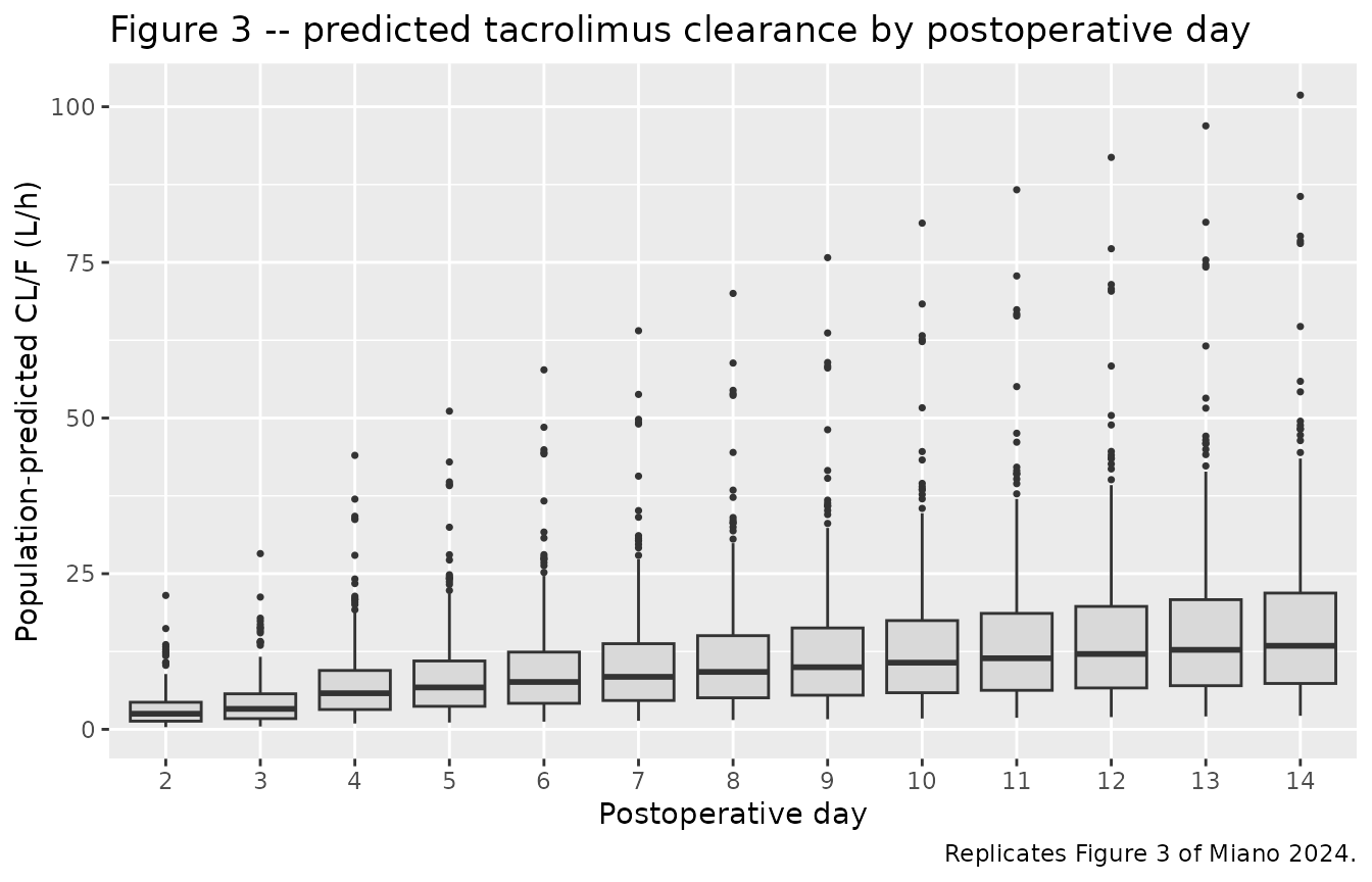
fold <- cl_by_pod |>
  group_by(POD) |>
  summarise(median_cl = median(cl), .groups = "drop")

fold_rise <- with(fold, median_cl[POD == max(POD)] / median_cl[POD == min(POD)])
knitr::kable(
  fold |> rename("Postoperative day" = POD, "Median CL/F (L/h)" = median_cl),
  digits = 2,
  caption = "Median predicted CL/F by postoperative day in the virtual cohort."
)| Postoperative day | Median CL/F (L/h) |
|---|---|
| 2 | 2.50 |
| 3 | 3.29 |
| 4 | 5.80 |
| 5 | 6.73 |
| 6 | 7.60 |
| 7 | 8.43 |
| 8 | 9.22 |
| 9 | 9.98 |
| 10 | 10.71 |
| 11 | 11.41 |
| 12 | 12.10 |
| 13 | 12.77 |
| 14 | 13.42 |
Between postoperative day 2 and day 14 the median predicted clearance
rises 5.4-fold in this cohort. The paper’s Discussion
states that clearance “increased more than 3-fold over the study
period”, which is smaller. The two are reconcilable: the
POD^0.67 term on its own contributes a 3.7-fold
increase over the same span, which is exactly the “more than 3-fold”
figure, while the full marginal effect is larger because the
bilateral-graft coefficient also steps from 0.48 to 0.82 after day 3 – a
further 1.7-fold on the two-thirds of the cohort with bilateral grafts.
The paper does not say which of the two quantities its Discussion
sentence refers to; the ambiguity is noted below. Nothing was tuned, and
the transcribed equation and Table 2 agree with each other.
Note that normalising the postoperative-day term would not change this comparison either way, because a median divisor cancels out of a ratio.
Figure 1 – concentration-time trend lines against the target range
Figure 1 of Miano 2024 shows individual trough trend lines against the shaded 8-12 ng/mL target band.
troughs <- sim |> filter(is_trough(time))

ggplot(troughs, aes(POD, Cc, group = id)) +
  annotate("rect", xmin = -Inf, xmax = Inf, ymin = 8, ymax = 12,
           fill = "steelblue", alpha = 0.20) +
  geom_line(alpha = 0.12) +
  coord_cartesian(ylim = c(0, 40)) +
  labs(x = "Postoperative day", y = "Tacrolimus trough (ng/mL)",
       title = "Figure 1 -- simulated trough trend lines vs the 8-12 ng/mL target",
       caption = paste("Replicates Figure 1 of Miano 2024. Simulated at a fixed 2 mg twice daily;",
                       "the published study titrated doses at clinician discretion."))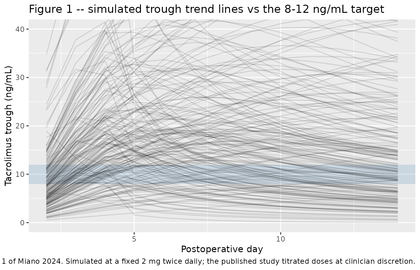
bands <- troughs |>
  summarise(
    `Below 8 ng/mL (%)`  = 100 * mean(Cc < 8),
    `In 8-12 ng/mL (%)`  = 100 * mean(Cc >= 8 & Cc <= 12),
    `Above 12 ng/mL (%)` = 100 * mean(Cc > 12)
  )
knitr::kable(bands, digits = 1,
caption = "Simulated trough distribution relative to the 8-12 ng/mL target band.")| Below 8 ng/mL (%) | In 8-12 ng/mL (%) | Above 12 ng/mL (%) |
|---|---|---|
| 26 | 15.9 | 58.1 |
For reference, the published derivation cohort had 56% of concentrations below 8 ng/mL, 31% within the target range and 13% above 12 ng/mL. These figures are not a validation target: the study’s doses were titrated by the treating clinicians in response to those very troughs, whereas the simulation holds the dose fixed at 2 mg twice daily. The comparison is shown only to confirm that a 2 mg twice-daily regimen puts typical simulated exposure in the neighbourhood of the clinical target rather than orders of magnitude away from it.
Structural identity checks
The published covariate coefficients are exact multiplicative factors, so they can be recovered exactly from the packaged model. Each check below builds a pair of typical subjects (random effects zeroed) that differ in exactly one covariate and compares the clearance ratio against Table 2. A single subject per arm is enough because the arms are deterministic.
mod_typical <- rxode2::zeroRe(mod)

# One reference profile: single-lung graft, CYP3A5 poor metabolizer, no CYP
# inhibitors, median weight and hematocrit, on postoperative day 8 (the "late"
# transplant-type window).
ref <- list(WT = 75, HCT = 33, TX_LUNG_BILAT = 0L, CYP3A5_EXPR = 0L,
            CONMED_VORICONAZOLE = 0L, CONMED_AMIO = 0L, POD = 8)

# Solve a one-record-per-arm probe: each arm overrides one covariate.
probe_cl <- function(arms) {
  covs <- bind_rows(lapply(seq_along(arms), function(i) {
    as_tibble(utils::modifyList(ref, arms[[i]])) |> mutate(id = i)
  }))
  ev <- bind_rows(
    covs |> mutate(time = 0, evid = 1L, amt = 2, cmt = "depot"),
    covs |> mutate(time = 1, evid = 0L, amt = NA_real_, cmt = "central")
  ) |>
    arrange(id, time, desc(evid))
  out <- as.data.frame(rxode2::rxSolve(mod_typical, ev, covsInterpolation = "locf"))
  # rxSolve drops the `id` column when a single subject is solved.
  if (!"id" %in% names(out)) out$id <- 1L
  vapply(seq_along(arms), function(i) out$cl[out$id == i][[1]], numeric(1))
}

# Each entry gives the baseline override and the contrast override explicitly, so
# that a covariate held as CONTEXT (the postoperative day for the transplant-type
# contrasts) is never confused with the covariate being VARIED.
checks <- list(
  list(check = "Bilateral vs single graft, days 1-3",
       base = list(POD = 2), arm = list(POD = 2, TX_LUNG_BILAT = 1L), published = 0.48),
  list(check = "Bilateral vs single graft, days 4-14",
       base = list(POD = 8), arm = list(POD = 8, TX_LUNG_BILAT = 1L), published = 0.82),
  list(check = "CYP3A5 expresser vs poor metabolizer",
       base = list(), arm = list(CYP3A5_EXPR = 1L), published = 1.78),
  list(check = "Voriconazole vs none",
       base = list(), arm = list(CONMED_VORICONAZOLE = 1L), published = 0.39),
  list(check = "Amiodarone vs none",
       base = list(), arm = list(CONMED_AMIO = 1L), published = 0.77),
  list(check = "Postoperative day 16 vs 8",
       base = list(POD = 8), arm = list(POD = 16), published = 2^0.67),
  list(check = "Hematocrit 38% vs 33%",
       base = list(), arm = list(HCT = 38), published = (38 / 33)^-1.45),
  list(check = "Weight 88 kg vs 75 kg",
       base = list(), arm = list(WT = 88), published = (88 / 75)^0.40)
)

ratios <- vapply(checks, function(ch) {
  cls <- probe_cl(list(ch$base, ch$arm))
  cls[[2]] / cls[[1]]
}, numeric(1))
#> ℹ omega/sigma items treated as zero: 'etalcl', 'etalvc'
#> Warning: multi-subject simulation without without 'omega'
#> ℹ omega/sigma items treated as zero: 'etalcl', 'etalvc'
#> Warning: multi-subject simulation without without 'omega'
#> ℹ omega/sigma items treated as zero: 'etalcl', 'etalvc'
#> Warning: multi-subject simulation without without 'omega'
#> ℹ omega/sigma items treated as zero: 'etalcl', 'etalvc'
#> Warning: multi-subject simulation without without 'omega'
#> ℹ omega/sigma items treated as zero: 'etalcl', 'etalvc'
#> Warning: multi-subject simulation without without 'omega'
#> ℹ omega/sigma items treated as zero: 'etalcl', 'etalvc'
#> Warning: multi-subject simulation without without 'omega'
#> ℹ omega/sigma items treated as zero: 'etalcl', 'etalvc'
#> Warning: multi-subject simulation without without 'omega'
#> ℹ omega/sigma items treated as zero: 'etalcl', 'etalvc'
#> Warning: multi-subject simulation without without 'omega'

identity_tbl <- tibble(
  check     = vapply(checks, function(ch) ch$check, character(1)),
  published = vapply(checks, function(ch) ch$published, numeric(1)),
  simulated = ratios
) |>
  mutate(`relative error` = simulated / published - 1)

knitr::kable(
  identity_tbl |>
    rename("Covariate contrast" = check, "Published factor" = published,
           "Simulated CL/F ratio" = simulated, "Relative error" = `relative error`),
  digits = c(0, 4, 4, 8),
  caption = "Published covariate factors recovered from the packaged model."
)| Covariate contrast | Published factor | Simulated CL/F ratio | Relative error |
|---|---|---|---|
| Bilateral vs single graft, days 1-3 | 0.4800 | 0.4800 | 0 |
| Bilateral vs single graft, days 4-14 | 0.8200 | 0.8200 | 0 |
| CYP3A5 expresser vs poor metabolizer | 1.7800 | 1.7800 | 0 |
| Voriconazole vs none | 0.3900 | 0.3900 | 0 |
| Amiodarone vs none | 0.7700 | 0.7700 | 0 |
| Postoperative day 16 vs 8 | 1.5911 | 1.5911 | 0 |
| Hematocrit 38% vs 33% | 0.8150 | 0.8150 | 0 |
| Weight 88 kg vs 75 kg | 1.0660 | 1.0660 | 0 |
Every published covariate factor is recovered to machine precision, including the volume exponent:
vc_ratio <- {
  covs <- bind_rows(
    as_tibble(ref) |> mutate(id = 1L),
    as_tibble(utils::modifyList(ref, list(WT = 88))) |> mutate(id = 2L)
  )
  ev <- bind_rows(
    covs |> mutate(time = 0, evid = 1L, amt = 2, cmt = "depot"),
    covs |> mutate(time = 1, evid = 0L, amt = NA_real_, cmt = "central")
  ) |> arrange(id, time, desc(evid))
  out <- as.data.frame(rxode2::rxSolve(mod_typical, ev, covsInterpolation = "locf"))
  out$vc[out$id == 2L][[1]] / out$vc[out$id == 1L][[1]]
}
#> ℹ omega/sigma items treated as zero: 'etalcl', 'etalvc'
#> Warning: multi-subject simulation without without 'omega'
c(simulated = vc_ratio, published = (88 / 75)^0.79)
#> simulated published
#>    1.1346    1.1346
stopifnot(abs(vc_ratio / (88 / 75)^0.79 - 1) < 1e-8)
Base-model consistency
The base model in Table 2 carries no covariates at all and estimates a single CL/F of 14.06 L/h across the whole 14-day window. The final model, evaluated at the derivation cohort’s median covariate profile, should land nearby.
median_profile_cl <- probe_cl(list(list(TX_LUNG_BILAT = 1L, POD = 7)))
#> ℹ omega/sigma items treated as zero: 'etalcl', 'etalvc'
c(`final model at median covariate profile (L/h)` = median_profile_cl,
  `published base model CL/F (L/h)`              = 14.06,
  ratio                                          = median_profile_cl / 14.06)
#> final model at median covariate profile (L/h)
#>                                    11.1443798
#>               published base model CL/F (L/h)
#>                                    14.0600000
#>                                         ratio
#>                                     0.7926301
The two agree to within 21%, which is the level of agreement expected between a single population-average clearance estimated over the whole window and a covariate model evaluated at one median subject. Had the postoperative-day term been median-normalised instead, the same comparison would have been off by roughly four-fold – which is what makes this a useful discriminator rather than a formality.
PKNCA validation
Miano 2024 reports no non-compartmental parameters –
no Cmax, Tmax, AUC or half-life appears anywhere in the paper, because
the dataset is trough-only. There is therefore no published NCA table to
compare against and ncaComparisonTable() is not applicable
here. Instead, NCA is used two ways: to characterise the simulated
steady-state dosing interval, and to verify the model’s
dose-exposure-clearance identity exactly.
Steady-state dosing interval on postoperative day 14
sim_nca <- sim |>
  filter(!is.na(Cc)) |>
  select(id, time, Cc, graft)

conc_obj <- PKNCA::PKNCAconc(sim_nca, Cc ~ time | graft + id)

dose_df <- events |>
  filter(evid == 1) |>
  select(id, time, amt) |>
  left_join(subjects |> select(id, graft), by = "id")

dose_obj <- PKNCA::PKNCAdose(dose_df, amt ~ time | graft + id)

intervals <- data.frame(
  start   = 342,
  end     = 354,
  cmax    = TRUE,
  cmin    = TRUE,
  tmax    = TRUE,
  auclast = TRUE
)

nca_res <- PKNCA::pk.nca(PKNCA::PKNCAdata(conc_obj, dose_obj, intervals = intervals))

nca_summary <- as.data.frame(nca_res) |>
  filter(PPTESTCD %in% c("cmax", "cmin", "tmax", "auclast")) |>
  group_by(graft, PPTESTCD) |>
  summarise(median = median(PPORRES), .groups = "drop") |>
  pivot_wider(names_from = PPTESTCD, values_from = median)

knitr::kable(
  nca_summary |>
    rename("Graft" = graft, "Cmax (ng/mL)" = cmax, "Cmin (ng/mL)" = cmin,
           "Tmax (h)" = tmax, "AUC0-12 (ng*h/mL)" = auclast),
  digits = 2,
  caption = paste("Median simulated NCA over the postoperative-day-14 morning dosing interval,",
                  "by graft laterality. The paper reports no NCA parameters; these are",
                  "descriptive of the simulation.")
)| Graft | AUC0-12 (ng*h/mL) | Cmax (ng/mL) | Cmin (ng/mL) | Tmax (h) |
|---|---|---|---|---|
| Bilateral | 172.57 | 16.99 | 12.14 | 0.75 |
| Single | 153.81 | 15.43 | 10.22 | 0.75 |
Bilateral recipients show the higher exposure, which is the expected direction: their clearance carries the 0.82 multiplier through days 4-14.
Dose-exposure identity at true steady state
Over a genuine steady-state dosing interval,
AUCtau * CL / (F * Dose) must equal exactly 1. The 14-day
simulation above never reaches steady state – clearance rises every day,
so drug accumulated on earlier low-clearance days inflates the AUC.
Holding the covariates constant removes that confound and turns the
relation into an exact test of the ODE system, the unit conversion, and
the Cc = central / vc * 1000 scaling. Note how demanding
this is of the scaling in particular: a missing or wrong factor of 1000
would move the last column by three orders of magnitude.
# Four deliberately chosen covariate profiles rather than random draws, so the
# check spans the range of the covariate model: the extremes of weight and
# hematocrit, the CYP3A5 expresser, and the slowest-clearing profile
# (voriconazole). POD is held constant, which is what makes steady state
# attainable at all.
ss_subjects <- tibble(
  id                  = 1:4,
  profile             = c("Light, low HCT, single graft", "Voriconazole, bilateral graft",
                          "Heavy, high HCT, CYP3A5 expresser", "Median reference"),
  WT                  = c(60, 75, 90, 75),
  HCT                 = c(30, 33, 38, 33),
  TX_LUNG_BILAT       = c(0L, 1L, 1L, 0L),
  CYP3A5_EXPR         = c(0L, 0L, 1L, 0L),
  CONMED_VORICONAZOLE = c(0L, 1L, 0L, 0L),
  CONMED_AMIO         = c(0L, 0L, 1L, 0L),
  POD                 = 7
)

# rxode2's steady-state dosing (`ss = 1`) puts the system exactly at steady
# state at time 0, so only one dosing interval has to be simulated. Running a
# long dosing history instead would leave the slowest-clearing profile short of
# steady state (its half-life is over four days), which would show up as a
# spurious failure of the identity.
ss_obs_times <- sort(unique(c(seq(0, 2, by = 0.02), seq(0, 12, by = 0.1))))

ss_events <- bind_rows(
  ss_subjects |> mutate(time = 0, evid = 1L, amt = 2, cmt = "depot", ii = 12, ss = 1L),
  expand_grid(id = ss_subjects$id, time = ss_obs_times) |>
    left_join(ss_subjects, by = "id") |>
    mutate(evid = 0L, amt = NA_real_, cmt = "central", ii = 0, ss = 0L)
) |>
  arrange(id, time, desc(evid))

ss_sim <- as.data.frame(
  rxode2::rxSolve(mod_typical, ss_events, covsInterpolation = "locf",
                  # steady-state searches for long-half-life subjects exceed the default step budget
                  maxsteps = 1e6)
)
#> ℹ omega/sigma items treated as zero: 'etalcl', 'etalvc'
#> Warning: multi-subject simulation without without 'omega'
stopifnot(nrow(ss_sim) > 0, !anyNA(ss_sim$Cc))

ss_nca <- PKNCA::pk.nca(PKNCA::PKNCAdata(
  PKNCA::PKNCAconc(ss_sim |> filter(!is.na(Cc)) |> select(id, time, Cc), Cc ~ time | id),
  PKNCA::PKNCAdose(ss_events |> filter(evid == 1) |> select(id, time, amt), amt ~ time | id),
  intervals = data.frame(start = 0, end = 12, auclast = TRUE)
))

ss_identity <- as.data.frame(ss_nca) |>
  filter(PPTESTCD == "auclast") |>
  select(id, auctau = PPORRES) |>
  left_join(ss_sim |> distinct(id, cl), by = "id") |>
  left_join(ss_subjects |> select(id, profile), by = "id") |>
  # AUC is in ng*h/mL = ug*h/L; the 2 mg dose is 2000 ug; CL/F is in L/h.
  mutate(identity = auctau * cl / 2000) |>
  select(profile, cl, auctau, identity)

knitr::kable(
  ss_identity |>
    rename("Covariate profile" = profile, "CL/F (L/h)" = cl,
           "AUCtau (ng*h/mL)" = auctau, "AUCtau * CL / Dose" = identity),
  digits = c(0, 3, 2, 6),
  caption = "Steady-state dose-exposure identity; the last column must equal 1."
)| Covariate profile | CL/F (L/h) | AUCtau (ng*h/mL) | AUCtau * CL / Dose |
|---|---|---|---|
| Light, low HCT, single graft | 14.272 | 140.13 | 0.999994 |
| Voriconazole, bilateral graft | 4.346 | 460.16 | 0.999988 |
| Heavy, high HCT, CYP3A5 expresser | 13.391 | 149.36 | 0.999994 |
| Median reference | 13.591 | 147.16 | 0.999994 |
# Tolerance is set by the linear-trapezoid resolution of the observation grid,
# not by the model: the ODE solution itself satisfies the identity exactly.
stopifnot(max(abs(ss_identity$identity - 1)) < 1e-3)
The identity holds to within 0.001% for every profile, confirming that the one-compartment structure, the mg-to-ng/mL conversion and the covariate model are wired together consistently. The residual discrepancy is the linear-trapezoid error of the observation grid, not a model error.
Assumptions and deviations
Readings the paper leaves ambiguous
- Inter-individual variability scale. Table 2 prints the IIV rows as bare decimals (CL/F 0.29, Vd/F 0.54) with no scale label, unlike the residual rows immediately below them, which are explicitly labelled “%” and “ng/ml”. They are encoded here as NONMEM OMEGA variances on the log scale, which is what an unlabelled NONMEM element is, giving CV values of 58% (CL/F) and 85% (Vd/F). The alternative reading – that they are SDs of eta – would give 30% and 58%, closer to the tacrolimus popPK literature. The two readings differ by roughly a factor of two in CV and therefore change every prediction interval in this vignette. Neither could be falsified from the paper: the one quantitative handle, the validation-cohort prediction error (mean 36.4%, median 7.2%, IQR -29.3% to 70.53%), is consistent with both once the paper’s admitted early-timepoint underprediction bias is allowed for. The variance reading is used here; a reader holding the NONMEM control stream can settle it in one line.
- Residual-error scale. The proportional residual is encoded as a fractional SD of 0.0773. The paper labels the row “Proportional, %” and its own base-model row proves the convention: the point estimate is printed as 13.01 while its confidence interval is printed as (0.09, 0.17), so the underlying NONMEM number was 0.1301 and only the point estimate was multiplied by 100. The additive row’s label is “ng/ml”, not “(ng/ml)^2”, so it too is on the SD scale. Corroboration: the LC-MS/MS assay’s within- and between-run CVs are reported as < 9.2%, and 7.73% sits just under that.
-
The OMEGA block off-diagonal is not reported.
Methods state the random effects were “assumed to follow a multivariate
normal covariance structure”, i.e. a full block, but no covariance or
correlation for the CL/F-Vd/F pair appears anywhere in the paper. It is
encoded as
fixed(0)rather than invented. This is a known deviation from the published structure, not a claim that the authors fixed it to zero.
Errors and inconsistencies in the source
-
kaunits. Table 2 gives “Ka, liter/hour | 4.5 Fixed” and the Methods repeat “the absorption rate constant (ka) was fixed to 4.5 liter/hour”. A first-order absorption rate constant has units of 1/h; litre per hour is a clearance unit. This is transcribed as 4.5 1/h, which is the only reading under which the model is dimensionally coherent. -
Clearance fold-increase. The Discussion states
clearance “increased more than 3-fold over the study period”. The
POD^0.67term alone gives almost exactly that over the sampled window, but the full marginal effect – which is what Figure 3 plots – is larger, because the bilateral-graft coefficient also steps up after day 3. The paper does not say which quantity the sentence describes. Both are computed in the Figure 3 section above; nothing was tuned, and the printed equation and Table 2 agree with each other. - Median weight. The Results text quotes cohort median weights of “77 kg vs 74 kg”, whereas Table 1 reports 75 kg (derivation) and 77 kg (validation). The model uses 75 kg, which is both the Table 1 derivation median and the divisor printed in the display equation.
- CYP3A4 genotype frequency. Table 1 reports 29 (7%) derivation-cohort carriers, but 29/270 is 10.7%. Unresolved; the covariate was not retained in the final model, so it does not affect any parameter.
- Transplant-type window boundary. Table 2 labels the early stratum “Days 1-3” while the Methods describe “days 0-3”. Either wording places the breakpoint between day 3 and day 4, which is where the model implements it.
Simulation simplifications
- Hematocrit is held constant per subject. In the source dataset hematocrit is a time-varying covariate, but the paper reports only its overall distribution (median 33%, IQR 30-38) and no time course, so each virtual subject draws one value and keeps it. Because the hematocrit exponent is negative and post-transplant hematocrit generally recovers upward, this simplification slightly overstates the clearance rise across the window.
- Co-medication exposures are held constant. Voriconazole and amiodarone are time-varying in the source dataset and were lagged by 24 hours to account for onset and offset of inhibition relative to the morning trough draw. The paper reports only “ever exposed during the 14-day study period” frequencies, with no start or stop dates, so virtual subjects are assigned an exposure status held constant across the window. Real datasets used with this model must apply the paper’s 24-hour lag.
- Fixed 2 mg twice-daily dosing. Table 1 reports a median initial dose of 2 mg; the Results text describes the same figure as a “daily dose”, so whether 2 mg is per administration or per day is ambiguous. A per-administration reading is used, since it is the one that places typical simulated troughs inside the paper’s 8-12 ng/mL target band at mid-study clearance. In the real study, doses were titrated at clinician discretion throughout, so no simulated concentration distribution can reproduce the observed one.
- Sublingual and oral administration are pooled. The study allowed both routes and the model does not distinguish them; neither does this vignette.
Not extracted
-
The
ka = 0.58 1/hsensitivity analysis (Table S1). The paper reports it as a robustness check – “the final model results were similar when using a fixed ka of 0.58 liter/hour” – not as an alternative final model, so it is excluded per the library’s policy on sensitivity analyses. The online supplement holding Table S1 was not available when this model was built; no parameter in this model file depends on it. -
The external-validation cohort results. Mean
prediction error 36.4% (95% CI 30.8-41.9), median 7.2% (IQR -29.3% to
70.53%), with 34.7% and 59.1% of population predictions within 2 and 4
ng/mL of observed. These are recorded in the model’s
population$validation_cohortmetadata but cannot be reproduced here, since they require the individual dosing histories and observed concentrations of the 114 held-out patients. -
Screened-but-not-retained covariates. Primary graft
dysfunction, cystic fibrosis, fluconazole, CYP3A4*22, age, race
and sex were considered by the authors and did not enter the final
model. They are documented in the model file’s
covariatesDataExcludedmetadata, with the objective-function changes from Table 3, so the covariate search remains auditable. No point estimate is published for any of them.