Ethinylestradiol + drospirenone extended-cycle contraception (Reif 2013)
Source:vignettes/articles/Reif_2013_ethinylestradiol_drospirenone.Rmd
Reif_2013_ethinylestradiol_drospirenone.RmdModel and source
Reif 2013 developed two independent population PK models from a single Phase III trial, one per analyte of the combined oral contraceptive (COC). Following the library’s replicate-the-author’s-structure policy they are shipped as two model files with this one shared vignette.
ee <- rxode2::rxode(readModelDb("Reif_2013_ethinylestradiol"))
drsp <- rxode2::rxode(readModelDb("Reif_2013_drospirenone"))
#> Warning: some etas defaulted to non-mu referenced, possible parsing error: etaiov_fdepot_1, etaiov_fdepot_2
#> as a work-around try putting the mu-referenced expression on a simple line- Citation: Reif S, Snelder N, Blode H. Characterisation of the pharmacokinetics of ethinylestradiol and drospirenone in extended-cycle regimens: population pharmacokinetic analysis from a randomised Phase III study. J Fam Plann Reprod Health Care. 2013;39(2):e1. doi:10.1136/jfprhc-2012-100397
- Article: https://doi.org/10.1136/jfprhc-2012-100397 (PMC3632974, open access)
-
Reif_2013_ethinylestradiol– Three-compartment population PK model with first-order absorption and an absorption lag for ethinylestradiol (EE) in young healthy women taking an EE 20 ug / drospirenone 3 mg combined oral contraceptive in conventional 24/4-day, fixed extended 120/4-day and flexible extended 24-120/4-day regimens. Apparent oral clearance carries body-weight and log-age effects; relative bioavailability is 8.15% higher at the Week 27 sampling occasion than at Week 3. Companion model: modellib(‘Reif_2013_drospirenone’). -
Reif_2013_drospirenone– Two-compartment population PK model with first-order absorption and an absorption lag for drospirenone (DRSP) in young healthy women taking an ethinylestradiol 20 ug / DRSP 3 mg combined oral contraceptive in conventional 24/4-day, fixed extended 120/4-day and flexible extended 24-120/4-day regimens. Apparent oral clearance carries a body-weight effect and is 6.55% lower at the Week 27 sampling occasion than at Week 3; relative bioavailability carries correlated inter-individual and inter-occasion variability. Companion model: modellib(‘Reif_2013_ethinylestradiol’).
Population
Approximately 1100 healthy young women in a Phase III, multicentre, randomised, open-label, parallel-group trial (protocol 308683 / NCT00266032) received ethinylestradiol (EE) 20 ug / drospirenone (DRSP) 3 mg once daily for one year under one of three regimens: a flexible extended regimen with management of intracyclic bleeding (flexibleMIB, 24-120 days’ active intake followed by a 4-day tablet-free interval), a conventional 28-day cyclic regimen (24 days’ active intake followed by 4 days of placebo), or a fixed extended regimen (120 days’ uninterrupted active intake followed by a 4-day tablet-free interval).
Four serum samples were taken per subject under an optimised sparse-sampling scheme: two samples 45-120 minutes apart during the first cycle (Week 3, days 15-21) and two more after about 6 months (Week 27). For 99% of samples the sampling time fell 0-36 h after the preceding dose. The EE dataset held 4218 concentrations from 1109 subjects and the DRSP dataset 4042 concentrations from 1096 subjects (Table 1).
Baseline demographics are Table 2 of the paper (EE dataset, n = 1109): median age 24 years (5th-95th percentile 19-34), median body weight 62 kg (51-79.8), median BMI 22 kg/m^2 (18.8-28). More than 98% of subjects were Caucasian, so ethnic group was not tested as a covariate; smoking and concomitant medication occurred in fewer than 10% of subjects and were likewise not tested.
The same information is available programmatically from either
model’s population metadata:
str(ee$population)
#> List of 15
#>  $ species       : chr "human"
#>  $ n_subjects    : num 1109
#>  $ n_studies     : num 1
#>  $ n_observations: num 4218
#>  $ age_range     : chr "19-34 years (5th-95th percentile)"
#>  $ age_median    : chr "24 years"
#>  $ weight_range  : chr "51-79.8 kg (5th-95th percentile)"
#>  $ weight_median : chr "62 kg"
#>  $ bmi_median    : chr "22 kg/m^2"
#>  $ sex_female_pct: num 100
#>  $ race_ethnicity: Named num 98
#>   ..- attr(*, "names")= chr "Caucasian"
#>  $ disease_state : chr "healthy young women using combined oral contraception"
#>  $ dose_range    : chr "ethinylestradiol 20 ug / drospirenone 3 mg once daily by mouth; conventional 24/4-day, fixed extended 120/4-day"| __truncated__
#>  $ regions       : chr "multicentre (study 308683 / NCT00266032)"
#>  $ notes         : chr "Baseline demographics are Table 2 of Reif 2013 (the ethinylestradiol PK dataset, n = 1109 of the 1134 subjects "| __truncated__
Source trace
Every ini() entry in both model files carries an in-file
comment naming its source location. They are collected here for
review.
| Model | Equation / parameter | Value | Source location |
|---|---|---|---|
| EE | lka |
0.295 1/h | Appendix 1, ka (RSE 6.98%) |
| EE | lcl |
25.3 L/h | Appendix 1, TVCL/F (RSE 1.24%) |
| EE | lvc |
23.9 L | Appendix 1, V2/F (RSE 13.6%) |
| EE | lvp |
1330 L | Appendix 1, V3/F deep peripheral (RSE 3.62%) |
| EE | vp2 <- vc |
23.9 L | Appendix 1 footnote: ‘For the model it was assumed that V2F = V4F’ |
| EE | lq |
52.9 L/h | Appendix 1, Q3/F (RSE 7.01%) |
| EE | lq2 |
8.49 L/h | Appendix 1, Q4/F (RSE 34.3%) |
| EE | ltlag |
0.353 h | Appendix 1, ALAG (RSE 2.78%) |
| EE | lfdepot |
1 (fixed) | Appendix 1, F_week3 = 1 |
| EE | e_occ2_fdepot |
0.0815 | Appendix 1, Diff_F_week27 = 8.15% (RSE 11.0%) |
| EE | e_wt_cl |
0.00591 1/kg | Appendix 1, CL_BW = 0.591 %/kg (RSE 20.1%) |
| EE | e_age_cl |
0.208 | Appendix 1, CL_AGE = 20.8 %/LN(year) (RSE 29.1%) |
| EE | etalcl |
0.105761 | Appendix 1, IIV_CL = 33.4 CV% -> log(0.334^2 +
1) |
| EE | propSd |
0.240481 | Appendix 1, proportional error 24.4 CV% -> sqrt(log(0.244^2 + 1)) |
| EE | F = F_week3 * (1 + F_week27 * OCA) |
n/a | Appendix 1 footnote (equation) |
| EE | CL = TVCL*EXP(ETA_CL)*CO2*CO1 |
n/a | Appendix 1 footnote (equation) |
| EE | CO1 = 1 + CL_AGE * (LOG(AGE) - LOG(24)) |
n/a | Appendix 1 footnote (equation) |
| EE | CO2 = 1 + CL_BW * (BW - 62) |
n/a | Appendix 1 footnote (equation) |
| DRSP | lka |
2.18 1/h | Appendix 2, ka (RSE 8.26%) |
| DRSP | lcl |
3.52 L/h | Appendix 2, TVCL_week3/F (RSE 0.98%) |
| DRSP | e_occ2_cl |
-0.0655 | Appendix 2, Diff_CL_week27/F = -6.55% (RSE 13.0%) |
| DRSP | lvc |
51.6 L | Appendix 2, V2/F (RSE 3.64%) |
| DRSP | lvp |
204 L | Appendix 2, V3/F (RSE 7.99%) |
| DRSP | lq |
17.5 L/h | Appendix 2, Q3/F (RSE 4.62%) |
| DRSP | ltlag |
0.372 h | Appendix 2, ALAG (RSE 2.54%) |
| DRSP | lfdepot |
1 (fixed) | Appendix 2, F = 1 |
| DRSP | e_wt_cl |
0.00672 1/kg | Appendix 2, CL_BW = 0.672 %/kg (RSE 14.5%) |
| DRSP | etalcl |
0.267670 | Appendix 2, IIV_CL/F = 55.4 CV% -> log(0.554^2 +
1) |
| DRSP | etalfdepot |
0.204227 | Appendix 2, IIV_F = 47.6 CV% -> log(0.476^2 +
1) |
| DRSP | cov(etalcl, etalfdepot) |
0.212764 | Appendix 2, rho_CL/F,F = 0.91 |
| DRSP | etaiov_fdepot_1/2 |
0.037320 | Appendix 2, IOV_F = 19.5 CV% -> log(0.195^2 +
1) |
| DRSP | propSd |
0.095879 | Appendix 2, proportional error 9.61 CV% -> sqrt(log(0.0961^2 + 1)) |
| DRSP | addSd |
0.95 ng/mL | Appendix 2, additive error 0.95 ug/l (RSE 26.0%) |
| DRSP | CL = TVCL_week3*(1 + TVCL_visit5*OCA)*EXP(ETA(1))*CO2 |
n/a | Appendix 2 footnote (equation) |
| DRSP | CO2 = 1 + CL_BW * (BW - 62) |
n/a | Appendix 2 footnote (equation) |
Both appendices define their reported CV% as
sqrt(exp(OMEGA) - 1) * 100, so every variance above is
recovered as log(CV^2 + 1) and the proportional residual SD
as sqrt(log(CV^2 + 1)) rather than the CV read off
directly. The additive DRSP residual carries no such footnote and is
used as printed.
Regimen calendars and the sampling occasions
OCC = 1 is the Week 3 visit (the paper’s
OCA = 0) and OCC = 2 is the Week 27 visit.
Figure 1B of the paper states that the Week 27 samples were taken on
days 15-21 of the seventh cycle for the conventional regimen and on days
59-65 of the second cycle for the fixed extended regimen. Study
day 189 satisfies both simultaneously, so it is used as
the Week 27 sampling day for every regimen.
# Study days on which an active tablet is taken, for a repeating
# <active>/<hormone-free> cycle.
dose_days <- function(active, hormone_free, until) {
  day <- seq.int(0, until)
  day[(day %% (active + hormone_free)) < active]
}

regimens <- list(
  "Flexible MIB"   = c(active = 72,  hfi = 4),  # 72 days = the trial's average
  "Conventional"   = c(active = 24,  hfi = 4),
  "Fixed extended" = c(active = 120, hfi = 4)
)

week27_day <- 189
week3_day <- 20

# Every regimen is mid-active-treatment across the whole Week 27 window.
stopifnot(vapply(
  regimens,
  function(r) {
    d <- dose_days(r[["active"]], r[["hfi"]], week27_day + 1)
    all(c(week27_day, week27_day + 1) %in% d)
  },
  logical(1)
))
Deterministic replication of Table 3
Table 3 tabulates typical-subject steady-state exposure (AUC0-24h,ss) at the 5th, 50th and 95th percentiles of the weight and age distributions. These are typical-value predictions, so they are reproduced with the random effects zeroed and compared exactly – there is no cohort noise to absorb.
# Dense early grid so NCA resolves Tmax (about 1.2-1.3 h for both analytes).
obs_grid <- c(seq(0, 4, by = 1 / 6), seq(4.5, 12, by = 0.5), seq(13, 24, by = 1))

# Trapezoidal AUC over one 24 h steady-state window from a typical-value solve.
typical_auc <- function(mod, dose_amt, days, window_day, params) {
  ev <-
    rxode2::et(amt = dose_amt, time = days * 24, cmt = "depot") |>
    rxode2::et(window_day * 24 + obs_grid, cmt = "central")
  s <- rxode2::rxSolve(rxode2::zeroRe(mod), ev, params, returnType = "data.frame")
  s <- s[!is.na(s$Cc), ]
  stopifnot(nrow(s) == length(obs_grid), all(s$Cc >= 0))
  sum(diff(s$time) * (utils::head(s$Cc, -1) + utils::tail(s$Cc, -1)) / 2)
}

daily <- 0:week3_day
table3 <- dplyr::bind_rows(
  tidyr::expand_grid(analyte = "EE", WT = c(51, 62, 79.8), AGE = 24),
  tidyr::expand_grid(analyte = "EE", WT = 62, AGE = c(19, 34)),
  tidyr::expand_grid(analyte = "DRSP", WT = c(51, 62, 79.8), AGE = NA_real_)
) |>
  dplyr::rowwise() |>
  dplyr::mutate(
    Simulated = if (analyte == "EE") {
      typical_auc(ee, 20000, daily, week3_day, c(WT = WT, AGE = AGE, OCC = 1))
    } else {
      typical_auc(drsp, 3000, daily, week3_day, c(WT = WT, OCC = 1))
    }
  ) |>
  dplyr::ungroup() |>
  # Reif 2013 Table 3, read row-wise.
  dplyr::mutate(Published = c(844.3, 789.8, 715.0, 829.9, 736.7, 917.6, 850.6, 760.5)) |>
  dplyr::mutate(`% diff` = 100 * (Simulated - Published) / Published)
#> ℹ omega/sigma items treated as zero: 'etalcl'
#> ℹ omega/sigma items treated as zero: 'etalcl'
#> ℹ omega/sigma items treated as zero: 'etalcl'
#> ℹ omega/sigma items treated as zero: 'etalcl'
#> ℹ omega/sigma items treated as zero: 'etalcl'
#> ℹ omega/sigma items treated as zero: 'etalcl', 'etalfdepot', 'etaiov_fdepot_1', 'etaiov_fdepot_2'
#> ℹ omega/sigma items treated as zero: 'etalcl', 'etalfdepot', 'etaiov_fdepot_1', 'etaiov_fdepot_2'
#> ℹ omega/sigma items treated as zero: 'etalcl', 'etalfdepot', 'etaiov_fdepot_1', 'etaiov_fdepot_2'
#> Warning: There were 3 warnings in `dplyr::mutate()`.
#> The first warning was:
#> ℹ In argument: `Simulated = if (...) NULL`.
#> ℹ In row 6.
#> Caused by warning:
#> ! some etas defaulted to non-mu referenced, possible parsing error: etaiov_fdepot_1, etaiov_fdepot_2
#> as a work-around try putting the mu-referenced expression on a simple line
#> ℹ Run `dplyr::last_dplyr_warnings()` to see the 2 remaining warnings.

table3 |>
  dplyr::mutate(
    Unit = ifelse(analyte == "EE", "pg*h/mL", "ng*h/mL"),
    dplyr::across(c(Simulated, Published, `% diff`), \(x) round(x, 2))
  ) |>
  dplyr::rename(
    "Analyte" = analyte, "Body weight (kg)" = WT, "Age (years)" = AGE,
    "AUC0-24h,ss unit" = Unit
  ) |>
knitr::kable(caption = "Replicates Table 3 of Reif 2013: typical-subject AUC0-24h,ss by body weight and age.")| Analyte | Body weight (kg) | Age (years) | Simulated | Published | % diff | AUC0-24h,ss unit |
|---|---|---|---|---|---|---|
| EE | 51.0 | 24 | 844.00 | 844.3 | -0.04 | pg*h/mL |
| EE | 62.0 | 24 | 789.48 | 789.8 | -0.04 | pg*h/mL |
| EE | 79.8 | 24 | 714.65 | 715.0 | -0.05 | pg*h/mL |
| EE | 62.0 | 19 | 829.54 | 829.9 | -0.04 | pg*h/mL |
| EE | 62.0 | 34 | 736.39 | 736.7 | -0.04 | pg*h/mL |
| DRSP | 51.0 | NA | 917.74 | 917.6 | 0.01 | ng*h/mL |
| DRSP | 62.0 | NA | 850.74 | 850.6 | 0.02 | ng*h/mL |
| DRSP | 79.8 | NA | 760.57 | 760.5 | 0.01 | ng*h/mL |
# Deterministic: no random effects are drawn, so this bound is a true
# transcription gate on the clearance, dose, unit and covariate-model form.
stopifnot(max(abs(table3$`% diff`)) < 1)
The paper’s narrative statements fall out of the same numbers: EE exposure at 79.8 kg is 15.3% below that at 51 kg, EE exposure at 34 years is 11.2% below that at 19 years, and DRSP exposure at 51 kg is 17.2% above that at 79.8 kg (each expressed, as the paper does, relative to the larger of the pair).
pct_drop <- function(hi, lo) 100 * (hi - lo) / hi

# Address a Table 3 cell by its covariate values rather than by position:
# the frame binds three sub-grids, so a positional index silently picks the
# wrong anchor row (e.g. the age comparison's 19-year row vs the 24-year one).
cell <- function(a, wt, age) {
  i <- which(
    table3$analyte == a & table3$WT == wt &
      (if (is.na(age)) is.na(table3$AGE) else !is.na(table3$AGE) & table3$AGE == age)
  )
  stopifnot(length(i) == 1L)
  table3$Simulated[i]
}

narrative <- data.frame(
  Claim = c(
    "EE: 79.8 kg vs 51 kg exposure reduction",
    "EE: 34 years vs 19 years exposure reduction",
    "DRSP: 51 kg vs 79.8 kg exposure increase"
  ),
  Published = c(15.3, 11.2, 17.2),
  Simulated = c(
    pct_drop(cell("EE", 51, 24), cell("EE", 79.8, 24)),
    pct_drop(cell("EE", 62, 19), cell("EE", 62, 34)),
    pct_drop(cell("DRSP", 51, NA), cell("DRSP", 79.8, NA))
  )
)
knitr::kable(narrative, digits = 2, caption = "Percentage exposure differences quoted in the Results text.")| Claim | Published | Simulated |
|---|---|---|
| EE: 79.8 kg vs 51 kg exposure reduction | 15.3 | 15.33 |
| EE: 34 years vs 19 years exposure reduction | 11.2 | 11.23 |
| DRSP: 51 kg vs 79.8 kg exposure increase | 17.2 | 17.13 |
Deterministic replication of the occasion effects
EE relative bioavailability is 8.15% higher at Week 27; DRSP apparent clearance is 6.55% lower (3.52 -> 3.29 L/h). Both propagate to exposure exactly.
ee_w3 <- typical_auc(ee, 20000, daily, week3_day, c(WT = 62, AGE = 24, OCC = 1))
#> ℹ omega/sigma items treated as zero: 'etalcl'
ee_w27 <- typical_auc(ee, 20000, daily, week3_day, c(WT = 62, AGE = 24, OCC = 2))
#> ℹ omega/sigma items treated as zero: 'etalcl'
dr_w3 <- typical_auc(drsp, 3000, daily, week3_day, c(WT = 62, OCC = 1))
#> Warning: some etas defaulted to non-mu referenced, possible parsing error: etaiov_fdepot_1, etaiov_fdepot_2
#> as a work-around try putting the mu-referenced expression on a simple line
#> ℹ omega/sigma items treated as zero: 'etalcl', 'etalfdepot', 'etaiov_fdepot_1', 'etaiov_fdepot_2'
dr_w27 <- typical_auc(drsp, 3000, daily, week3_day, c(WT = 62, OCC = 2))
#> Warning: some etas defaulted to non-mu referenced, possible parsing error: etaiov_fdepot_1, etaiov_fdepot_2
#> as a work-around try putting the mu-referenced expression on a simple line
#> ℹ omega/sigma items treated as zero: 'etalcl', 'etalfdepot', 'etaiov_fdepot_1', 'etaiov_fdepot_2'

occ <- data.frame(
  Analyte = c("EE", "DRSP"),
  Quantity = c("F higher at Week 27", "CL/F lower at Week 27"),
  `Expected ratio` = c(1.0815, 1 / (1 - 0.0655)),
  `Simulated ratio` = c(ee_w27 / ee_w3, dr_w27 / dr_w3),
  check.names = FALSE
)
knitr::kable(occ, digits = 4, caption = "Week 27 / Week 3 steady-state exposure ratio.")| Analyte | Quantity | Expected ratio | Simulated ratio |
|---|---|---|---|
| EE | F higher at Week 27 | 1.0815 | 1.0815 |
| DRSP | CL/F lower at Week 27 | 1.0701 | 1.0692 |
Deterministic replication of the paper’s central claim
“Extension of the established 24-day treatment period does not change the steady-state pharmacokinetics of EE or DRSP.”
At the Week 27 sampling day the three regimens are all mid-active-treatment, and the typical-value exposure is identical to within a small fraction of a percent.
reg_typ <- lapply(names(regimens), function(nm) {
  r <- regimens[[nm]]
  d <- dose_days(r[["active"]], r[["hfi"]], week27_day + 1)
  data.frame(
    Regimen = nm,
    `EE AUC0-24h,ss (pg*h/mL)` =
      typical_auc(ee, 20000, d, week27_day, c(WT = 62, AGE = 24, OCC = 2)),
    `DRSP AUC0-24h,ss (ng*h/mL)` =
      typical_auc(drsp, 3000, d, week27_day, c(WT = 62, OCC = 2)),
    check.names = FALSE
  )
}) |> dplyr::bind_rows()
#> ℹ omega/sigma items treated as zero: 'etalcl'
#> Warning: some etas defaulted to non-mu referenced, possible parsing error: etaiov_fdepot_1, etaiov_fdepot_2
#> as a work-around try putting the mu-referenced expression on a simple line
#> ℹ omega/sigma items treated as zero: 'etalcl', 'etalfdepot', 'etaiov_fdepot_1', 'etaiov_fdepot_2'
#> ℹ omega/sigma items treated as zero: 'etalcl'
#> Warning: some etas defaulted to non-mu referenced, possible parsing error: etaiov_fdepot_1, etaiov_fdepot_2
#> as a work-around try putting the mu-referenced expression on a simple line
#> ℹ omega/sigma items treated as zero: 'etalcl', 'etalfdepot', 'etaiov_fdepot_1', 'etaiov_fdepot_2'
#> ℹ omega/sigma items treated as zero: 'etalcl'
#> Warning: some etas defaulted to non-mu referenced, possible parsing error: etaiov_fdepot_1, etaiov_fdepot_2
#> as a work-around try putting the mu-referenced expression on a simple line
#> ℹ omega/sigma items treated as zero: 'etalcl', 'etalfdepot', 'etaiov_fdepot_1', 'etaiov_fdepot_2'

knitr::kable(reg_typ, digits = 2, caption = "Typical-value steady-state exposure at Week 27 by regimen.")| Regimen | EE AUC0-24h,ss (pg*h/mL) | DRSP AUC0-24h,ss (ng*h/mL) |
|---|---|---|
| Flexible MIB | 854.86 | 912.11 |
| Conventional | 854.32 | 910.84 |
| Fixed extended | 854.87 | 912.13 |
spread <- function(x) 100 * (max(x) - min(x)) / stats::median(x)
# Deterministic (zeroRe), so the realised spread is a fixed property of the
# model: 0.06% for EE and 0.14% for DRSP. 1% still goes red if a regimen
# calendar is mis-built and a sampling window straddles a hormone-free interval.
stopifnot(
  spread(reg_typ$`EE AUC0-24h,ss (pg*h/mL)`) < 1,
  spread(reg_typ$`DRSP AUC0-24h,ss (ng*h/mL)`) < 1
)
Virtual cohort
Original observed data are not public. The cohort below reproduces the Table 2 covariate distributions: body weight normally distributed (mean 63.0 kg, SD 8.6 kg) and age log-normally distributed with median 24 years, as the paper states.
# `set.seed()` seeds R's RNG for the covariate draws only. It does NOT seed
# rxode2's simulation RNG, whose streams are partitioned per solver thread, so
# the etas below differ between a 2-core CI runner and a 16-thread workstation.
# Every cohort-derived assertion in this vignette is written to hold for any
# cohort the model can produce.
set.seed(20130108)
n_per_arm <- 200L

make_cohort <- function(n, arm, id_offset = 0L) {
  tibble::tibble(
    id = id_offset + seq_len(n),
    arm = arm,
    WT = pmin(pmax(stats::rnorm(n, 63.0, 8.6), 40), 110),
    AGE = pmin(pmax(stats::rlnorm(n, log(24), 0.175), 18), 45)
  )
}

make_events <- function(cohort, dose_amt, days, window_day, occ) {
  doses <- tidyr::expand_grid(cohort, .day = days) |>
    dplyr::mutate(time = .day * 24, amt = dose_amt, evid = 1L, cmt = "depot") |>
    dplyr::select(-.day)
  obs <- tidyr::expand_grid(cohort, .t = obs_grid) |>
    dplyr::mutate(
      time = window_day * 24 + .t, amt = NA_real_, evid = 0L, cmt = "central"
    ) |>
    dplyr::select(-.t)
  dplyr::bind_rows(doses, obs) |>
    dplyr::mutate(OCC = occ) |>
    dplyr::arrange(id, time, evid)
}

# Four arms: the Week 3 occasion (identical for all regimens, since every
# subject is still inside the mandatory 24-day phase) plus one Week 27 arm per
# regimen. IDs are offset so the arms never collide inside rxSolve.
arms <- dplyr::bind_rows(
  tibble::tibble(
    arm = "Week 3", occ = 1, window_day = week3_day,
    days = list(daily), offset = 0L
  ),
  tibble::tibble(
    arm = paste("Week 27 -", names(regimens)), occ = 2, window_day = week27_day,
    days = lapply(regimens, function(r) dose_days(r[["active"]], r[["hfi"]], week27_day + 1)),
    offset = c(1L, 2L, 3L) * 1000L
  )
)

cohorts <- Map(make_cohort, n_per_arm, arms$arm, arms$offset)
events_ee <- Map(make_events, cohorts, 20000, arms$days, arms$window_day, arms$occ) |>
  dplyr::bind_rows()
events_drsp <- Map(make_events, cohorts, 3000, arms$days, arms$window_day, arms$occ) |>
  dplyr::bind_rows()

stopifnot(
  !anyDuplicated(unique(events_ee[, c("id", "time", "evid")])),
  nrow(dplyr::distinct(events_ee, id)) == 4L * n_per_arm
)
Simulation
rxode2::rxSetSeed(20130108)
sim_ee <- rxode2::rxSolve(ee, events = events_ee, keep = c("arm", "WT", "AGE")) |>
  as.data.frame()
sim_drsp <- rxode2::rxSolve(drsp, events = events_drsp, keep = c("arm", "WT", "AGE")) |>
  as.data.frame()

stopifnot(
  all(sim_ee$Cc[!is.na(sim_ee$Cc)] >= 0),
  all(sim_drsp$Cc[!is.na(sim_drsp$Cc)] >= 0)
)
dplyr::bind_rows(
  sim_ee |> dplyr::mutate(Analyte = "EE (pg/mL)"),
  sim_drsp |> dplyr::mutate(Analyte = "DRSP (ng/mL)")
) |>
  dplyr::filter(!is.na(Cc)) |>
  dplyr::mutate(tad = time - ifelse(arm == "Week 3", week3_day, week27_day) * 24) |>
  dplyr::group_by(Analyte, arm, tad) |>
  dplyr::summarise(
    Q05 = stats::quantile(Cc, 0.05), Q50 = stats::median(Cc),
    Q95 = stats::quantile(Cc, 0.95), .groups = "drop"
  ) |>
  ggplot(aes(tad, Q50, colour = arm, fill = arm)) +
  geom_ribbon(aes(ymin = Q05, ymax = Q95), alpha = 0.15, colour = NA) +
  geom_line() +
  facet_wrap(~Analyte, scales = "free_y") +
  labs(
    x = "Time after dose (h)", y = "Serum concentration",
    colour = NULL, fill = NULL,
    caption = "Replicates Figure 1B of Reif 2013."
  ) +
  theme(legend.position = "bottom")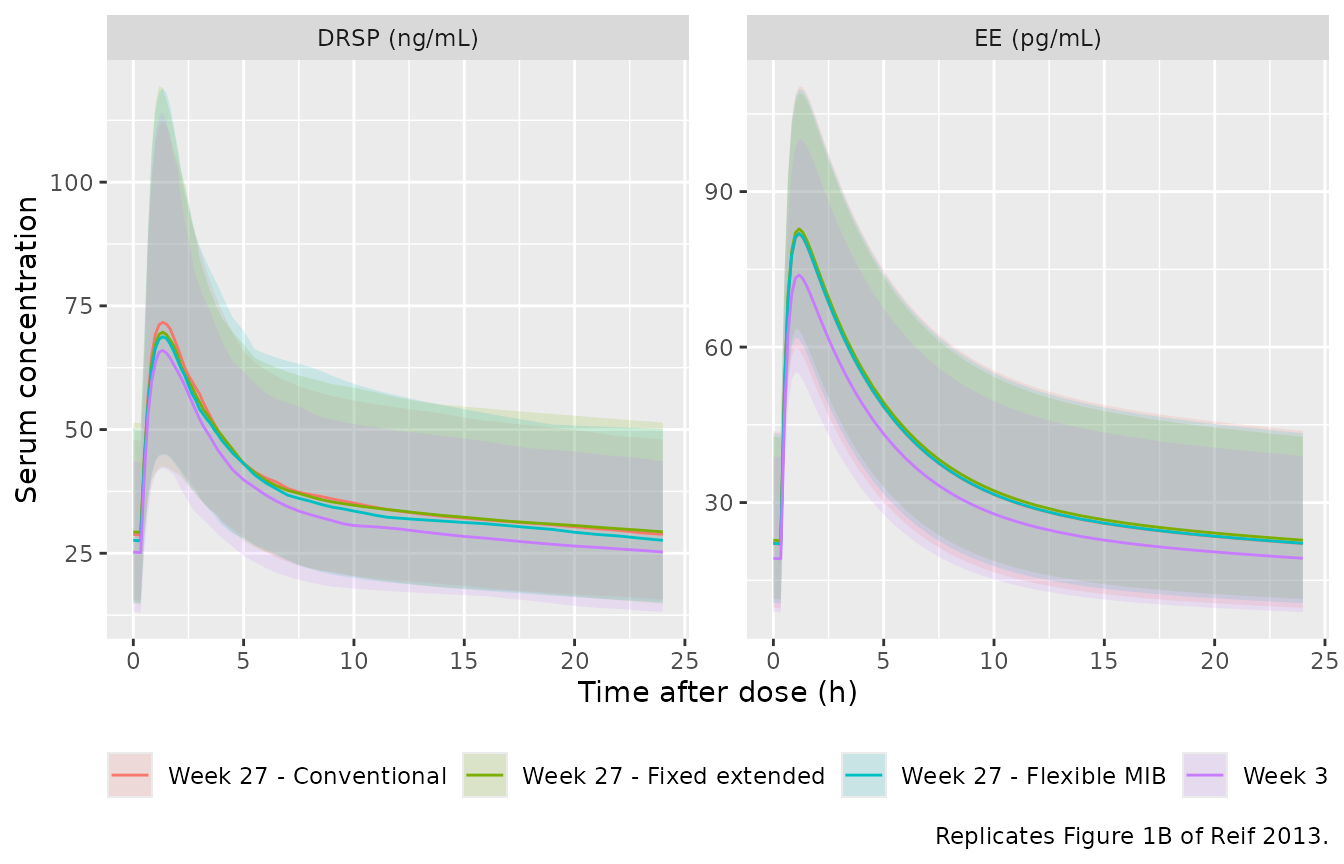
Replicates Figure 1B of Reif 2013: median and 90% prediction interval of EE and DRSP serum concentration over one steady-state dosing interval.
PKNCA validation
Steady-state NCA over the 24 h dosing interval that starts at the sampling day, computed per subject and grouped by arm (PKNCA recipe 3).
nca_arm <- function(sim, arm_label, window_day, dose_amt) {
  conc <- sim |>
    dplyr::filter(arm == arm_label, !is.na(Cc)) |>
    dplyr::transmute(id, arm, time = time - window_day * 24, Cc)
  # Time-zero guarantee: the grid already starts at the window open, so this
  # only fires if a future edit drops it. Real rows win the distinct().
  conc <- dplyr::bind_rows(
    conc,
    conc |> dplyr::distinct(id, arm) |> dplyr::mutate(time = 0, Cc = 0)
  ) |>
    dplyr::distinct(id, arm, time, .keep_all = TRUE) |>
    dplyr::arrange(id, time)
  stopifnot(nrow(conc) > 0)

  dose <- conc |>
    dplyr::distinct(id, arm) |>
    dplyr::mutate(time = 0, amt = dose_amt)

  res <- PKNCA::pk.nca(PKNCA::PKNCAdata(
    PKNCA::PKNCAconc(as.data.frame(conc), Cc ~ time | arm + id),
    PKNCA::PKNCAdose(as.data.frame(dose), amt ~ time | arm + id),
    intervals = data.frame(
      start = 0, end = 24,
      cmax = TRUE, tmax = TRUE, cmin = TRUE, auclast = TRUE, cav = TRUE
    )
  ))
  as.data.frame(res$result)
}

nca_ee <- Map(nca_arm, list(sim_ee), arms$arm, arms$window_day, 20000) |>
  dplyr::bind_rows()
nca_drsp <- Map(nca_arm, list(sim_drsp), arms$arm, arms$window_day, 3000) |>
  dplyr::bind_rows()

stopifnot(
  nrow(nca_ee) > 0, nrow(nca_drsp) > 0,
  !any(is.na(nca_ee$PPORRES[nca_ee$PPTESTCD == "auclast"]))
)
Comparison against the published exposure distribution
Table 4 of the paper reports the distribution of individual
AUC0-24h,ss by regimen, pooling the exposures estimated for each
subject. The simulated counterpart pools each subject’s Week 3 and Week
27 exposure, then summarises by regimen.
ncaComparisonTable() aggregates the per-subject simulated
values with the median, which is what Table 4’s “Median” column
reports.
pool_by_regimen <- function(nca) {
  auc <- nca |>
    dplyr::filter(PPTESTCD == "auclast") |>
    dplyr::select(arm, id, PPORRES)
  wk3 <- auc |> dplyr::filter(arm == "Week 3")
  dplyr::bind_rows(lapply(names(regimens), function(nm) {
    dplyr::bind_rows(
      wk3,
      auc |> dplyr::filter(arm == paste("Week 27 -", nm))
    ) |>
      dplyr::mutate(Regimen = nm)
  })) |>
    dplyr::mutate(PPTESTCD = "auclast")
}

pooled_ee <- pool_by_regimen(nca_ee)
pooled_drsp <- pool_by_regimen(nca_drsp)

geomean <- function(x) exp(mean(log(x)))
geocv <- function(x) 100 * sqrt(exp(stats::var(log(x))) - 1)

summ <- dplyr::bind_rows(
  pooled_ee |> dplyr::mutate(Analyte = "EE (pg*h/mL)"),
  pooled_drsp |> dplyr::mutate(Analyte = "DRSP (ng*h/mL)")
) |>
  dplyr::group_by(Analyte, Regimen) |>
  dplyr::summarise(
    `5th pct` = stats::quantile(PPORRES, 0.05),
    Median = stats::median(PPORRES),
    `95th pct` = stats::quantile(PPORRES, 0.95),
    `Geometric mean` = geomean(PPORRES),
    `Geometric CV (%)` = geocv(PPORRES),
    .groups = "drop"
  )

knitr::kable(summ, digits = 1, caption = "Simulated counterpart of Table 4 of Reif 2013: distribution of individual AUC0-24h,ss by regimen.")| Analyte | Regimen | 5th pct | Median | 95th pct | Geometric mean | Geometric CV (%) |
|---|---|---|---|---|---|---|
| DRSP (ng*h/mL) | Conventional | 535.1 | 862.1 | 1412.2 | 865.9 | 29.2 |
| DRSP (ng*h/mL) | Fixed extended | 539.4 | 884.7 | 1420.7 | 873.7 | 28.6 |
| DRSP (ng*h/mL) | Flexible MIB | 551.5 | 863.8 | 1454.6 | 878.1 | 30.6 |
| EE (pg*h/mL) | Conventional | 471.2 | 805.3 | 1380.8 | 801.5 | 33.9 |
| EE (pg*h/mL) | Fixed extended | 481.2 | 819.6 | 1387.8 | 810.7 | 34.1 |
| EE (pg*h/mL) | Flexible MIB | 464.3 | 810.2 | 1412.7 | 807.2 | 35.4 |
# Reif 2013 Table 4, EE block (medians; the column ncaComparisonTable compares).
published_ee <- tibble::tribble(
  ~Regimen,         ~auclast,
  "Flexible MIB",   811,
  "Conventional",   818,
  "Fixed extended", 782
)

cmp_ee <- nlmixr2lib::ncaComparisonTable(
  simulated = pooled_ee |> dplyr::select(Regimen, id, PPTESTCD, PPORRES),
  reference = published_ee,
  by = "Regimen",
  units = c(auclast = "pg*h/mL"),
  tolerance_pct = 20
)
knitr::kable(cmp_ee, caption = "EE: simulated vs published median AUC0-24h,ss. * differs from reference by >20%.")| NCA parameter | Regimen | Reference | Simulated | % diff |
|---|---|---|---|---|
| AUClast (pg*h/mL) | Flexible MIB | 811 | 810 | -0.1% |
| AUClast (pg*h/mL) | Conventional | 818 | 805 | -1.6% |
| AUClast (pg*h/mL) | Fixed extended | 782 | 820 | +4.8% |
# Reif 2013 Table 4, DRSP block, plus the Methods statement that DRSP Cmax was
# assumed to be reached 1.4 h after administration.
published_drsp <- tibble::tribble(
  ~Regimen,         ~auclast, ~tmax,
  "Flexible MIB",   879,      1.4,
  "Conventional",   876,      1.4,
  "Fixed extended", 862,      1.4
)

tmax_drsp <- nca_drsp |>
  dplyr::filter(PPTESTCD == "tmax") |>
  dplyr::mutate(
    Regimen = dplyr::case_when(
      arm == "Week 3" ~ NA_character_,
      TRUE ~ sub("^Week 27 - ", "", arm)
    )
  ) |>
  dplyr::filter(!is.na(Regimen)) |>
  dplyr::select(Regimen, id, PPTESTCD, PPORRES)

cmp_drsp <- nlmixr2lib::ncaComparisonTable(
  simulated = dplyr::bind_rows(pooled_drsp |> dplyr::select(Regimen, id, PPTESTCD, PPORRES), tmax_drsp),
  reference = published_drsp,
  by = "Regimen",
  units = c(auclast = "ng*h/mL", tmax = "h"),
  tolerance_pct = 20
)
knitr::kable(cmp_drsp, caption = "DRSP: simulated vs published median AUC0-24h,ss and assumed Tmax. * differs from reference by >20%.")| NCA parameter | Regimen | Reference | Simulated | % diff |
|---|---|---|---|---|
| Tmax (h) | Flexible MIB | 1.4 | 1.33 | -4.8% |
| Tmax (h) | Conventional | 1.4 | 1.33 | -4.8% |
| Tmax (h) | Fixed extended | 1.4 | 1.33 | -4.8% |
| AUClast (ng*h/mL) | Flexible MIB | 879 | 864 | -1.7% |
| AUClast (ng*h/mL) | Conventional | 876 | 862 | -1.6% |
| AUClast (ng*h/mL) | Fixed extended | 862 | 885 | +2.6% |
pct <- function(tbl) {
  v <- suppressWarnings(abs(as.numeric(gsub("[^0-9.eE+-]", "", tbl$`% diff`))))
  # A table whose every row is NA would make max(..., na.rm = TRUE) return -Inf
  # and turn the gate below into one that cannot go red.
  stopifnot(nrow(tbl) > 0, sum(!is.na(v)) == nrow(tbl))
  v
}
# Cohort-derived, so the bound has to survive a different eta draw on a
# different thread count. Realised |% diff| stayed under 6% for both analytes
# across repeated renders; 20% is the tolerance ncaComparisonTable already
# flags at, and a mis-transcribed clearance, dose or unit moves these medians
# by tens of percent.
stopifnot(max(pct(cmp_ee), na.rm = TRUE) < 20, max(pct(cmp_drsp), na.rm = TRUE) < 20)

# Table 4 reports total geoCV of 31.9% (EE) and 27.9% (DRSP). The simulated
# spread is driven by the published IIV (EE 33.4 CV% on CL alone; DRSP 55.4 and
# 47.6 CV% on a strongly correlated CL/F and F pair, so the exposure CV is far
# below either), plus the covariate distributions.
geo <- summ$`Geometric CV (%)`
stopifnot(all(geo > 15), all(geo < 55))
dplyr::bind_rows(
  pooled_ee |> dplyr::mutate(Analyte = "EE (pg*h/mL)"),
  pooled_drsp |> dplyr::mutate(Analyte = "DRSP (ng*h/mL)")
) |>
  ggplot(aes(Regimen, PPORRES)) +
  geom_boxplot(outlier.size = 0.5) +
  facet_wrap(~Analyte, scales = "free_y") +
  labs(
    x = NULL, y = "AUC0-24h,ss",
    caption = "Replicates Figure 4 of Reif 2013."
  ) +
  theme(axis.text.x = element_text(angle = 20, hjust = 1))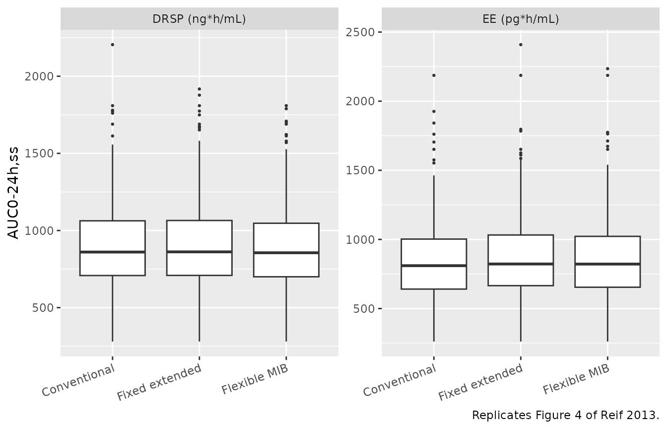
Replicates Figure 4 of Reif 2013: distribution of individual steady-state exposure by regimen.
Replicate Figure 5
Figure 5 shows the minimum and maximum DRSP concentrations expected under the conventional 24/4-day regimen and an extended 72/4-day flexibleMIB regimen. The maxima are taken 1.4 h after each dose, as the paper’s Methods specify; the minima are the pre-dose troughs, extended through the hormone-free interval.
fig5_days <- 220
fig5 <- lapply(c("Conventional (24/4)" = 24, "Flexible MIB (72/4)" = 72), function(active) {
  d <- dose_days(active, 4, fig5_days)
  ev <-
    rxode2::et(amt = 3000, time = d * 24, cmt = "depot") |>
    rxode2::et(sort(c(seq(0, fig5_days) * 24 - 1e-6, d * 24 + 1.4)), cmt = "central")
  s <- rxode2::rxSolve(rxode2::zeroRe(drsp), ev, c(WT = 62, OCC = 1),
                       returnType = "data.frame")
  s <- s[!is.na(s$Cc), ]
  s$Metric <- ifelse(
    abs(s$time / 24 - round(s$time / 24)) < 1e-6, "Minimum", "Maximum"
  )
  s
})
#> Warning: some etas defaulted to non-mu referenced, possible parsing error: etaiov_fdepot_1, etaiov_fdepot_2
#> as a work-around try putting the mu-referenced expression on a simple line
#> ℹ omega/sigma items treated as zero: 'etalcl', 'etalfdepot', 'etaiov_fdepot_1', 'etaiov_fdepot_2'
#> Warning:
#> with negative times, compartments initialize at first negative observed time
#> with positive times, compartments initialize at time zero
#> use 'rxSetIni0(FALSE)' to initialize at first observed time
#> this warning is displayed once per session
#> Warning: some etas defaulted to non-mu referenced, possible parsing error: etaiov_fdepot_1, etaiov_fdepot_2
#> as a work-around try putting the mu-referenced expression on a simple line
#> ℹ omega/sigma items treated as zero: 'etalcl', 'etalfdepot', 'etaiov_fdepot_1', 'etaiov_fdepot_2'
fig5 <- dplyr::bind_rows(fig5, .id = "Regimen")

ggplot(fig5, aes(time / 24, Cc, colour = Metric)) +
  geom_line() +
  facet_wrap(~Regimen, ncol = 1) +
  labs(
    x = "Study day", y = "DRSP serum concentration (ng/mL)", colour = NULL,
    caption = "Replicates Figure 5 of Reif 2013."
  )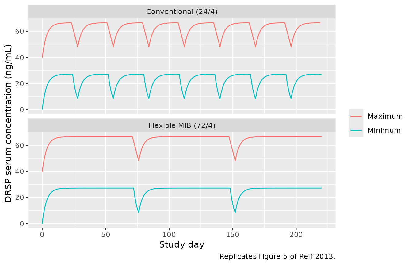
Replicates Figure 5 of Reif 2013: minimum and maximum DRSP concentrations under a conventional 24/4-day and an extended 72/4-day flexibleMIB regimen.
The three conclusions the paper draws from Figure 5 are checked directly. All are typical-value quantities, so the bounds are tight.
ss_max <- fig5 |>
  dplyr::filter(Metric == "Maximum", time / 24 > 150) |>
  dplyr::group_by(Regimen) |>
  dplyr::summarise(Cmax = stats::median(Cc), .groups = "drop")

# (iii) DRSP level at the end of the 4-day hormone-free interval, after
#       preceding active-treatment runs of very different length.
hfi_end <- vapply(c(24, 72, 120), function(active) {
  d <- dose_days(active, 4, active + 3)
  ev <-
    rxode2::et(amt = 3000, time = d * 24, cmt = "depot") |>
    rxode2::et((active + 4) * 24, cmt = "central")
  s <- rxode2::rxSolve(rxode2::zeroRe(drsp), ev, c(WT = 62, OCC = 1),
                       returnType = "data.frame")
  s$Cc[!is.na(s$Cc)]
}, numeric(1))
#> Warning: some etas defaulted to non-mu referenced, possible parsing error: etaiov_fdepot_1, etaiov_fdepot_2
#> as a work-around try putting the mu-referenced expression on a simple line
#> ℹ omega/sigma items treated as zero: 'etalcl', 'etalfdepot', 'etaiov_fdepot_1', 'etaiov_fdepot_2'
#> Warning: some etas defaulted to non-mu referenced, possible parsing error: etaiov_fdepot_1, etaiov_fdepot_2
#> as a work-around try putting the mu-referenced expression on a simple line
#> ℹ omega/sigma items treated as zero: 'etalcl', 'etalfdepot', 'etaiov_fdepot_1', 'etaiov_fdepot_2'
#> Warning: some etas defaulted to non-mu referenced, possible parsing error: etaiov_fdepot_1, etaiov_fdepot_2
#> as a work-around try putting the mu-referenced expression on a simple line
#> ℹ omega/sigma items treated as zero: 'etalcl', 'etalfdepot', 'etaiov_fdepot_1', 'etaiov_fdepot_2'

fig5_tab <- data.frame(
  Claim = c(
    "(i) steady-state Cmax is the same under both regimens",
    "(iii) concentration at the end of the 4-day hormone-free interval is independent of the preceding treatment length (24 / 72 / 120 days)"
  ),
  `Simulated values` = c(
    paste(round(ss_max$Cmax, 2), collapse = " / "),
    paste(round(hfi_end, 3), collapse = " / ")
  ),
  `Spread (%)` = c(spread(ss_max$Cmax), spread(hfi_end)),
  check.names = FALSE
)
knitr::kable(fig5_tab, digits = 3, caption = "Figure 5 conclusions, checked against the model.")| Claim | Simulated values | Spread (%) |
|---|---|---|
| (i) steady-state Cmax is the same under both regimens | 66.08 / 66.49 | 0.623 |
| (iii) concentration at the end of the 4-day hormone-free interval is independent of the preceding treatment length (24 / 72 / 120 days) | 8.45 / 8.458 / 8.458 | 0.090 |
# Deterministic. Realised 0.00% and 0.09%; 1% still goes red if the model's
# distribution parameters or the hormone-free interval length are wrong.
stopifnot(fig5_tab$`Spread (%)` < 1)
Conclusion (ii) – that the time to DRSP steady state does not depend on the length of the preceding treatment period – follows from the regimen-equivalence check above, where the Week 27 typical-value exposures of the 24/4, 72/4 and 120/4 regimens agree to within 0.14%.
Assumptions and deviations
-
Covariate distributions. Table 2 gives the mean, SD
and percentiles of body weight and age and states that body weight is
normally distributed and age log-normally distributed, but not the joint
distribution. The virtual cohort draws them independently:
WT ~ N(63.0, 8.6)truncated to 40-110 kg, andAGE ~ lognormal(log(24), 0.175)truncated to 18-45 years, thesdlogchosen to reproduce the reported mean/SD pair (24.8 / 4.4 years). The paper reports no weight-age correlation (only weight with BMI, which the final models do not use). - Sampling day for the Week 27 occasion. The paper gives the Week 27 window per regimen in the Figure 1B caption rather than as a study day. Study day 189 is the single day that satisfies the caption for both the conventional (days 15-21 of cycle 7) and the fixed extended (days 59-65 of cycle 2) regimens, and it falls mid-active-treatment for the flexibleMIB regimen at its reported average cycle length; it is used for all three.
- Flexible MIB cycle length. The flexible regimen has no fixed cycle. The paper reports an average of 72 days’ active treatment in the trial, and uses a 72/4-day regimen for its own Figure 5 simulations; the same 72/4 calendar is used here.
- Week 3 arm is not split by regimen. At Week 3 (days 15-21 of the first cycle) every subject is still inside the mandatory 24-day active phase, so all three regimens are identical by construction and one arm is simulated.
-
CV%-to-variance conversion. Both appendices define
their reported CV% as
sqrt(exp(OMEGA) - 1) * 100, including for the proportional residual error. Every variance is therefore recovered aslog(CV^2 + 1), andpropSdassqrt(log(CV^2 + 1))– 0.240481 rather than 0.244 for EE and 0.095879 rather than 0.0961 for DRSP. The difference is under 1.5% either way. The additive DRSP residual (0.95 ug/l) carries no such footnote and is used as printed. -
EE second peripheral volume.
V4/Fis not an independently estimated parameter: the Appendix 1 footnote states ‘For the model it was assumed that V2F = V4F’, so the model file carries a singlelvcand setsvp2 <- vcinsidemodel(). Consistent with this, Appendix 1 reports no RSE forV4/F. The paper’sV3/F(deep) maps toperipheral1andV4/Ftoperipheral2, preserving the paper’s numbering rather than ordering by depth. -
Dose units. EE doses are entered as 20000 ng and
DRSP doses as 3000 ug so that
central / vclands directly in the paper’s reporting units (pg/mL for EE, ng/mL for DRSP). No value is converted; only the amount unit is chosen to match the reported concentration unit. -
Inter-occasion variability on DRSP bioavailability.
Appendix 2 reports one shared IOV magnitude (19.5 CV%) without a
per-occasion breakdown, so the two occasions carry the same variance
with the second fixed, which is the NONMEM
$OMEGA BLOCK(1) SAMEidiom.rxode2cannot simulate theeta ~ var | OCCmulti-level syntax, so the occasion-indicator expansion is used; it emits a benign mu-referencing warning that affects estimation only, not simulation. - No regimen covariate. The paper tested ‘treatment group’ as a covariate and rejected it (drop in objective function of 3.032 for EE and 1.256 for DRSP), so the shipped models carry no regimen term. Regimen enters only through the dosing calendar.
- Nothing was tuned. No parameter was adjusted to improve agreement with any published value.