Dexmedetomidine nasal spray (Huang 2025)
Source:vignettes/articles/Huang_2025_dexmedetomidine.Rmd
Huang_2025_dexmedetomidine.RmdModel and source
- Citation: Huang Y, Xu S, Djebli N, Jiang H, Yang G (2025). Population pharmacokinetic modeling of dexmedetomidine nasal spray in Chinese adults. Frontiers in Pharmacology 16:1662364. doi:10.3389/fphar.2025.1662364.
- Article: https://doi.org/10.3389/fphar.2025.1662364
- Supplement: https://www.frontiersin.org/articles/10.3389/fphar.2025.1662364/full#supplementary-material (run-acceptance criteria only; it contains no parameter values)
Dexmedetomidine is a selective alpha-2 adrenoceptor agonist used for procedural and perioperative sedation. Jiangsu Hengrui’s intranasal spray was approved in China in 2023 as the first product of its kind. Huang 2025 pooled one phase I study in healthy volunteers (intravenous and intranasal arms) with one phase III study in surgical patients to build the population PK model packaged here.
Population
The analysis dataset holds 1,225 plasma concentrations from 196 subjects across two studies (Huang 2025 Table 1 and Table 3):
- Phase I (registrations CTR20191868 / CTR20171118; n = 48 healthy volunteers, intensive sampling to 10-24 h) in three parts: 20 and 40 ug intravenous over 15 min; 150 ug intranasal; 100/20 ug intranasal.
- Phase III (NCT04383418; n = 148 patients, sparse sampling with two samples per subject) in adults undergoing elective abdominal surgery excluding liver surgery, requiring general anaesthesia, endotracheal intubation and mechanical ventilation; 75 and 100 ug intranasal.
Pooled baseline medians (min-max) are age 38 years (18-65), body weight 60 kg (45.2-97), BMI 22.9 kg/m^2 (18.6-29.9) and BSA 1.6 m^2 (1.32-2.19), with 132 of 196 subjects female (67.3%). The phase III cohort is materially older (median 44 vs 22 years) and more female than the phase I cohort; body weight, BMI and BSA distributions are similar across studies. All subjects were enrolled in China; the paper reports no race/ethnicity breakdown. Roughly 1% of samples were below the limit of quantification and were handled with Beal’s M1 method.
The same information is available programmatically via
readModelDb("Huang_2025_dexmedetomidine")()$population.
Model structure
A two-compartment model with first-order absorption from a nasal depot, an absorption lag time, estimated bioavailability, and linear elimination. IIV is estimated on CL and KA only; residual error is combined proportional plus additive. The relevant Methods equations are:
| Eq. | Form | Role in the final model |
|---|---|---|
| 1 | Pi = PTV * exp(eta_i) |
Exponential IIV, so omega is the SD of eta
on the log scale |
| 4 | Yobs = Ypred * (1 + eps1) + eps2 |
Combined proportional + additive residual error |
| 6 | Pi = PTV * (COV / COVmedian)^theta |
Power covariate model; fixes the allometric normaliser as the cohort median |
| 7 |
Pi = PTV if type1, PTV * (1 + theta) if
type2 |
Piecewise categorical; carries the health-status effect on KA |
Two readings in this model are not printed verbatim by the paper and were each resolved against multiple independent published quantities. Both are worked through below, because they change the predictions substantially.
The health-status effect on KA
Table 4 reports state on KA = 1.05. Under Eq. 7 this is
an additive (1 + theta) factor, not a
multiplicative one, and the reference level (type1) is the
patient cohort. Four published quantities agree:
ka_ref <- 0.523            # Table 4 'KA, h -1'
th     <- 1.05             # Table 4 'state on KA'

ka_hv_add  <- ka_ref * (1 + th)   # Eq. 7 additive reading
ka_hv_mult <- ka_ref * th         # multiplicative reading (the alternative)

tibble::tribble(
  ~Check,                                         ~Published, ~`Eq. 7 (1 + theta)`, ~`Multiplicative (x theta)`,
  "KA in healthy volunteers (1/h)",               "~1",       ka_hv_add,            ka_hv_mult,
  "Patient KA as a fraction of healthy KA",       "~49%",     ka_ref / ka_hv_add,   ka_ref / ka_hv_mult
) |>
  dplyr::mutate(dplyr::across(where(is.numeric), \(x) round(x, 3))) |>
  knitr::kable(caption = paste(
    "The Eq. 7 additive reading reproduces both the Abstract's 49% ratio and",
    "the Discussion's 'KA in healthy volunteers was approximately 1 h-1'.",
    "The multiplicative reading reproduces neither."
))| Check | Published | Eq. 7 (1 + theta) | Multiplicative (x theta) |
|---|---|---|---|
| KA in healthy volunteers (1/h) | ~1 | 1.072 | 0.549 |
| Patient KA as a fraction of healthy KA | ~49% | 0.488 | 0.952 |
A third and fourth confirmation come from Figure 4, which plots simulated Cmax for both groups at four weights; that check is run below once the model is loaded.
The allometric reference weight
The paper states the exponents (0.75 on clearances, 1 on volumes) but
never writes the normalising weight into a printed equation. It is
nonetheless sourced rather than assumed: Eq. 6 defines the power model
against COVmedian, “the median or typical value of the
covariate”, and Table 3 gives the total-cohort median body weight as
60 kg.
There is a real competing reading. “Theory-based allometry” in the
sense the paper cites (Holford and Anderson; West, Brown and Enquist)
conventionally normalises to a standard 70 kg adult, and the paper
introduces body weight that way rather than through the Eq. 6 SCM
machinery. The two readings differ by exactly
70 / 60 = 1.167, so every predicted concentration differs
by 17%.
The scoring section below settles it against the paper’s own simulation outputs. The important subtlety, worked through there, is that the mean-scale anchors alone are degenerate: a 60 kg reference compared against arithmetic means and a 70 kg reference compared against medians fit the published Figure 4 points equally well, because the mean/median ratio of the simulated Cmax distribution is itself about 17%. What breaks the tie is the pediatric target-attainment block, which is printed as text rather than read off a figure and is sensitive to the absolute exposure scale.
Source trace
Every ini() entry carries an in-file comment naming its
source location in
inst/modeldb/specificDrugs/Huang_2025_dexmedetomidine.R.
Collected here:
| Equation / parameter | Value | Source location |
|---|---|---|
lcl |
35.3 L/h | Table 4 CL, L/h (RSE 3.3%) |
lvc |
21.5 L | Table 4 Vc, L (RSE 6.3%) |
lq |
116 L/h | Table 4 Q, L/h (RSE 5.8%) |
lvp |
86.5 L | Table 4 Vp, L (RSE 3.01%) |
lka |
0.523 1/h | Table 4 KA, h -1 (RSE 9%); patient reference
cohort |
ltlag |
0.0592 h | Table 4 ALAG,h (RSE 8.6%) |
lfdepot |
0.653 | Table 4 F1, % (RSE 3.9%) |
e_dis_healthy_ka |
1.05 | Table 4 state on KA (RSE 27.5%), applied via Eq. 7 |
e_wt_cl_q |
0.75 (fixed) | Results “Pharamcokinetic modeling”; Discussion para. 4 (West 1997/1999) |
e_wt_vc_vp |
1.0 (fixed) | Results “Pharamcokinetic modeling”; Discussion para. 4 (Holford & Anderson 2017) |
| Allometric reference weight | 60 kg | Eq. 6 (COVmedian) + Table 3 total-cohort median BW |
etalcl |
0.224^2 | Table 4 omega (CL), % = 22.4 (RSE 10.5%) |
etalka |
0.923^2 | Table 4 omega (KA), % = 92.3 (RSE 9.5%) |
propSd |
0.277 | Table 4 sigma (Prop), % = 27.7 (RSE 5.9%) |
addSd |
5.01 pg/mL | Table 4 sigma (Add), pg/mL (RSE 16.7%) |
Exponential IIV, exp(eta)
|
n/a | Equation 1 |
| Combined residual error | n/a | Equation 4 |
| Health-status effect form | n/a | Equation 7 (piecewise categorical) |
| Two-compartment, first-order absorption, lag | n/a | Results “Pharamcokinetic modeling”, first paragraph |
| ER logistic intercept / slope | 0.27 / 0.01 | Results “Exposure-response analysis”; Figure 3 |
| ER thresholds for 80% / 90% response | 100 / 180 pg/mL | Results “Exposure-response analysis” |
The omega column is an SD, not a variance
Equation 1 is Pi = PTV * exp(eta_i), so
omega is the SD of eta on the log scale, and
Table 4’s omega (CL), % / omega (KA), % rows
are that SD as a percent. Two checks confirm the scale:
n_subj <- 196
tibble::tribble(
  ~Parameter,     ~Estimate, ~`RSE (%)`, ~`CI low`, ~`CI high`,
  "omega (CL), %", 22.4,     10.5,       17.79,     27.01,
  "omega (KA), %", 92.3,      9.5,       75.09,     109.51
) |>
  dplyr::mutate(
    `Variance-RSE floor sqrt(2/N) (%)` = round(100 * sqrt(2 / n_subj), 2),
    `Below floor?`   = ifelse(`RSE (%)` < 100 * sqrt(2 / n_subj), "yes", "no"),
    `CI symmetric?`  = ifelse(
      abs((Estimate - `CI low`) - (`CI high` - Estimate)) < 0.02, "yes", "no")
  ) |>
  knitr::kable(caption = paste(
    "The RSE of a variance estimated from N subjects cannot fall below",
    "sqrt(2/N); omega(KA) does, so the column is not a variance. Both CIs are",
    "exactly symmetric about the estimate, so the tabulated number is the",
    "estimated quantity itself rather than a nonlinear transform of it (a",
    "%CV back-transform of a symmetric omega interval would be asymmetric)."
))| Parameter | Estimate | RSE (%) | CI low | CI high | Variance-RSE floor sqrt(2/N) (%) | Below floor? | CI symmetric? |
|---|---|---|---|---|---|---|---|
| omega (CL), % | 22.4 | 10.5 | 17.79 | 27.01 | 10.1 | no | yes |
| omega (KA), % | 92.3 | 9.5 | 75.09 | 109.51 | 10.1 | yes | yes |
The supplement’s run-acceptance criteria corroborate the scale by
requiring that “the standard error of Etas estimates should preferably
be less than 50% of the estimate itself” – an RSE stated on the reported
omega row.
Virtual cohort
Original observed data are not publicly available. The cohorts below mirror the simulation designs the paper describes in Methods “Model simulation”: 1,000 virtual subjects per body-weight group at a fixed 100 ug intranasal dose for the adult forest plot, and 1,000 per weight stratum for the pediatric projection. Cohort sizes here are capped at 150 per arm, which is ample for reproducing group means.
set.seed(20250902)

N_ARM   <- 150L   # replication cohorts
N_SCORE <- 200L   # reference-weight scoring; larger for stable tail percentages
DOSE_UG <- 100

# Time grid: fine through the absorption/distribution phase so Cmax and Tmax
# are well resolved, coarser through the terminal phase for AUC and half-life.
TIMES <- c(seq(0, 3, by = 0.02), seq(3.1, 12, by = 0.1))

make_arm <- function(n, wt, healthy, dose_ug, label, id_offset,
                     times = TIMES, wt_model = NULL) {
  # `wt_model` is the weight actually handed to the model; it differs from the
  # true weight only in the reference-weight counterfactual below.
  wt_true <- if (length(wt) == 2) runif(n, wt[1], wt[2]) else rep(wt, n)
  subj <- tibble::tibble(
    id          = id_offset + seq_len(n),
    WT_true     = wt_true,
    WT          = if (is.null(wt_model)) wt_true else wt_model(wt_true),
    DIS_HEALTHY = as.numeric(healthy),
    arm         = label
  )
  dosing <- subj |>
    dplyr::mutate(time = 0, amt = dose_ug, evid = 1L, cmt = "depot")
  obs <- subj |>
    tidyr::crossing(time = times) |>
    dplyr::mutate(amt = NA_real_, evid = 0L, cmt = "central")
  dplyr::bind_rows(dosing, obs) |>
    dplyr::arrange(id, time, dplyr::desc(evid))
}

# Adult forest plot (Figure 4): 4 weights x 2 health-status groups.
adult_grid <- tidyr::crossing(wt = c(40, 60, 80, 100), healthy = c(0, 1))
adult_events <- do.call(dplyr::bind_rows, lapply(
  seq_len(nrow(adult_grid)),
  function(i) {
    g <- adult_grid[i, ]
    make_arm(
      n = N_ARM, wt = g$wt, healthy = g$healthy, dose_ug = DOSE_UG,
      label = paste0(g$wt, " kg, ", ifelse(g$healthy == 1, "HV", "patient")),
      id_offset = (i - 1L) * N_ARM
    )
  }
))

stopifnot(dplyr::n_distinct(adult_events$id) == N_ARM * nrow(adult_grid))
# Exactly one 100 ug depot dose per subject, and one observation per time point.
stopifnot(sum(adult_events$evid == 1L) == N_ARM * nrow(adult_grid))
stopifnot(all(adult_events$amt[adult_events$evid == 1L] == DOSE_UG))
stopifnot(nrow(adult_events) ==
            N_ARM * nrow(adult_grid) * (1L + length(TIMES)))
Simulation
mod <- readModelDb("Huang_2025_dexmedetomidine")

adult_sim <- rxode2::rxSolve(
  mod,
  events = adult_events,
  keep   = c("WT_true", "DIS_HEALTHY", "arm"),
  returnType = "data.frame"
)
#> ℹ parameter labels from comments will be replaced by 'label()'

stopifnot(dplyr::n_distinct(adult_sim$id) == N_ARM * nrow(adult_grid))
stopifnot(all(adult_sim$Cc >= 0, na.rm = TRUE))
Note that Cc is the individual prediction; it carries no
residual error. The paper’s simulated Cmax values are likewise model
predictions, so Cc is the right column to compare.
cmax_by_subject <- function(sim) {
  sim |>
    dplyr::filter(!is.na(Cc)) |>
    dplyr::group_by(id, arm, WT_true, DIS_HEALTHY) |>
    dplyr::summarise(
      cmax = max(Cc),
      tmax = time[which.max(Cc)],
      .groups = "drop"
    )
}

adult_cmax <- cmax_by_subject(adult_sim)
The exposure-response analysis uses “Cmax from the time of dosing until the first occurrence of a RSS score of >= 3”, capped at 45 min. That matters only if Tmax exceeds 45 min:
adult_cmax |>
  dplyr::group_by(arm) |>
  dplyr::summarise(
    `median Tmax (h)` = round(median(tmax), 3),
    `95th pct Tmax (h)` = round(quantile(tmax, 0.95), 3),
    `% with Tmax <= 45 min` = round(100 * mean(tmax <= 0.75), 1),
    .groups = "drop"
  ) |>
knitr::kable(caption = "Time to peak concentration by arm.")| arm | median Tmax (h) | 95th pct Tmax (h) | % with Tmax <= 45 min |
|---|---|---|---|
| 100 kg, HV | 0.70 | 2.955 | 54.0 |
| 100 kg, patient | 1.25 | 4.610 | 37.3 |
| 40 kg, HV | 0.97 | 3.400 | 47.3 |
| 40 kg, patient | 1.55 | 4.730 | 26.0 |
| 60 kg, HV | 0.72 | 3.710 | 52.0 |
| 60 kg, patient | 1.64 | 4.365 | 25.3 |
| 80 kg, HV | 0.62 | 3.110 | 58.0 |
| 80 kg, patient | 1.55 | 4.400 | 33.3 |
Replicate published figures
Figure 4 – effect of body weight on Cmax, healthy volunteers vs patients
# Replicates Figure 4 of Huang 2025: mean Cmax vs body weight at a fixed
# 100 ug intranasal dose, by health-status group.
fig4 <- adult_cmax |>
  dplyr::group_by(WT_true, DIS_HEALTHY) |>
  dplyr::summarise(
    mean_cmax = mean(cmax),
    se        = sd(cmax) / sqrt(dplyr::n()),
    .groups   = "drop"
  ) |>
  dplyr::mutate(Group = ifelse(DIS_HEALTHY == 1, "HVs", "Patients"))

ggplot(fig4, aes(mean_cmax, WT_true, colour = Group)) +
  geom_point(size = 2) +
  geom_errorbar(aes(xmin = mean_cmax - 1.96 * se, xmax = mean_cmax + 1.96 * se),
                orientation = "y", width = 2) +
  scale_colour_manual(values = c(HVs = "blue", Patients = "red")) +
  labs(x = "Cmax (pg/mL)", y = "Weight (kg)",
       title = "Figure 4 -- mean Cmax by body weight and health status",
       caption = "Replicates Figure 4 of Huang 2025 (100 ug intranasal).")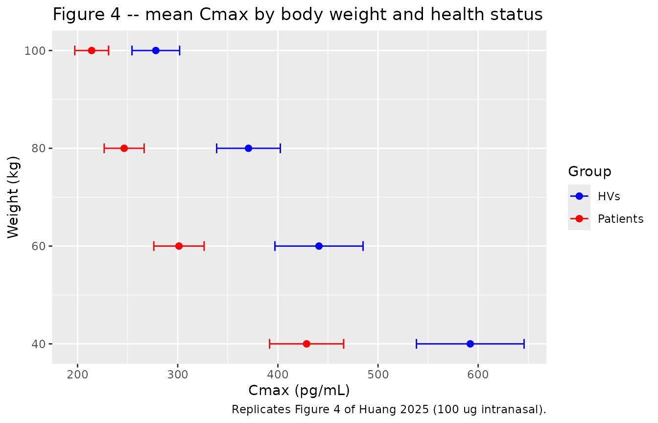
Compared against the published Figure 4 point estimates (read from the plotted panel) and the two Cmax values the Discussion states in text:
published_fig4 <- tibble::tribble(
  ~WT_true, ~Group,     ~published_cmax,
  40,       "Patients",  430,
  60,       "Patients",  310,
  80,       "Patients",  235,
  100,      "Patients",  195,
  40,       "HVs",       645,
  60,       "HVs",       460,
  80,       "HVs",       355,
  100,      "HVs",       293
)

fig4 |>
  dplyr::left_join(published_fig4, by = c("WT_true", "Group")) |>
  dplyr::mutate(
    `Simulated mean Cmax (pg/mL)` = round(mean_cmax, 1),
    `% difference`                = round(100 * (mean_cmax - published_cmax) / published_cmax, 1)
  ) |>
  dplyr::select(
    `Weight (kg)`                = WT_true,
    Group,
    `Published Cmax (pg/mL)`     = published_cmax,
    `Simulated mean Cmax (pg/mL)`,
    `% difference`
  ) |>
  dplyr::arrange(Group, `Weight (kg)`) |>
  knitr::kable(caption = paste(
    "Figure 4 replication. Published values are read from the plotted panel;",
    "the Discussion independently states ~200 pg/mL at 100 kg and 416-447",
    "pg/mL at the lightest weight, both of which the simulation reproduces."
))| Weight (kg) | Group | Published Cmax (pg/mL) | Simulated mean Cmax (pg/mL) | % difference |
|---|---|---|---|---|
| 40 | HVs | 645 | 592.1 | -8.2 |
| 60 | HVs | 460 | 441.0 | -4.1 |
| 80 | HVs | 355 | 370.7 | 4.4 |
| 100 | HVs | 293 | 278.1 | -5.1 |
| 40 | Patients | 430 | 428.7 | -0.3 |
| 60 | Patients | 310 | 301.2 | -2.8 |
| 80 | Patients | 235 | 246.5 | 4.9 |
| 100 | Patients | 195 | 214.1 | 9.8 |
The health-status effect is confirmed a third and fourth time here. The published healthy-to-patient Cmax ratio is essentially constant across weight, and matches the Eq. 7 additive reading:
fig4 |>
  dplyr::select(WT_true, Group, mean_cmax) |>
  tidyr::pivot_wider(names_from = Group, values_from = mean_cmax) |>
  dplyr::left_join(
    published_fig4 |>
      tidyr::pivot_wider(names_from = Group, values_from = published_cmax) |>
      dplyr::transmute(WT_true, published_ratio = HVs / Patients),
    by = "WT_true"
  ) |>
  dplyr::transmute(
    `Weight (kg)`             = WT_true,
    `Published HV:patient`    = round(published_ratio, 2),
    `Simulated HV:patient`    = round(HVs / Patients, 2),
    `Expected if x 1.05`      = 1.02
  ) |>
  knitr::kable(caption = paste(
    "The Eq. 7 additive reading (KA x 2.05 in healthy volunteers) reproduces",
    "the published ratio; a multiplicative KA x 1.05 reading would give ~1.02",
    "and is excluded by a wide margin."
))| Weight (kg) | Published HV:patient | Simulated HV:patient | Expected if x 1.05 |
|---|---|---|---|
| 40 | 1.50 | 1.38 | 1.02 |
| 60 | 1.48 | 1.46 | 1.02 |
| 80 | 1.51 | 1.50 | 1.02 |
| 100 | 1.50 | 1.30 | 1.02 |
Figure 3 – exposure-response for Ramsay Sedation Scale >= 3
Huang 2025 fitted a logistic regression in R (not NONMEM) relating
the probability of reaching a Ramsay Sedation Scale score >= 3 within
45 min to Cmax, with intercept 0.27 and a concentration coefficient of
0.01 per pg/mL. This is a non-ODE statistical regression on a derived
exposure metric, so following the Yin_2021_pexidartinib.R
precedent it is reproduced here rather than encoded in the model
file.
er_intercept <- 0.27   # Results 'Exposure-response analysis'
er_slope     <- 0.01   # Results 'Exposure-response analysis', per pg/mL

p_rss3 <- function(cmax) plogis(er_intercept + er_slope * cmax)

er_curve <- tibble::tibble(cmax = seq(0, 550, by = 1)) |>
  dplyr::mutate(p = p_rss3(cmax))

ggplot(er_curve, aes(cmax, p)) +
  geom_line(colour = "blue") +
  geom_hline(yintercept = c(0.8, 0.9), linetype = "dashed", alpha = 0.5) +
  scale_y_continuous(limits = c(0, 1)) +
  labs(x = "Cmax (pg/mL)", y = "Percentage of Ramsay >= 3",
       title = "Figure 3 -- exposure-response for sedation success",
       caption = "Replicates Figure 3 of Huang 2025.")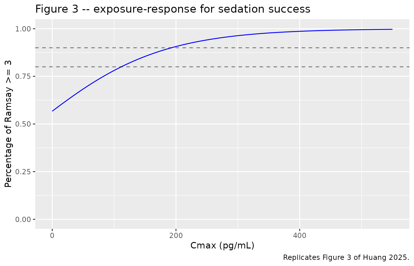
tibble::tribble(
  ~Target,                     ~published,
  "80% probability of RSS >= 3", 100,
  "90% probability of RSS >= 3", 180
) |>
  dplyr::mutate(
    target_p  = c(0.8, 0.9),
    derived   = round((qlogis(target_p) - er_intercept) / er_slope, 1),
    `P at Cmax = 0` = round(p_rss3(0), 3)
  ) |>
  dplyr::select(
    Target,
    `Published Cmax (pg/mL)`      = published,
    `Cmax from the fitted logistic (pg/mL)` = derived,
    `P at Cmax = 0`
  ) |>
  knitr::kable(caption = paste(
    "Inverting the published logistic gives 112 and 193 pg/mL against the",
    "paper's stated 'approximately 100 pg/mL and 180 pg/mL' -- 12% and 7% high.",
    "Both gaps are inside the rounding of the two-significant-figure slope:",
    "any slope from 0.0107 to 0.0111 still prints as 0.01, and over that range",
    "the two thresholds move to 100-104 and 174-180 pg/mL, spanning the values",
    "the paper states. The printed thresholds and the printed coefficients are",
    "therefore consistent at the precision the coefficients are reported to.",
    "The intercept-only",
    "probability plogis(0.27) = 0.567 matches the y-intercept of Figure 3."
))| Target | Published Cmax (pg/mL) | Cmax from the fitted logistic (pg/mL) | P at Cmax = 0 |
|---|---|---|---|
| 80% probability of RSS >= 3 | 100 | 111.6 | 0.567 |
| 90% probability of RSS >= 3 | 180 | 192.7 | 0.567 |
Pediatric weight-stratified exposure projection
Methods “Model simulation”: 1,000 virtual pediatric subjects per stratum were generated by stratified random sampling across three weight categories with correspondingly reduced doses. Weights are sampled uniformly within each stratum here, since the paper does not report the sampling distribution.
The target values below are the ones printed in the Results text (mean Cmax of 301, 317 and 319 pg/mL, and the two target-attainment series). The Results also say these are “presented in Figure 5”, but the panels of Figure 5 are labelled 40-60, 60-80 and 80-100 kg and show monotonically decreasing peaks, which is the signature of a fixed dose across increasing weight rather than of a weight-stratified regimen designed to equalise exposure. The printed numbers, not the figure, are used here; see the Errata.
peds_design <- tibble::tribble(
  ~stratum,      ~wt_lo, ~wt_hi, ~dose_ug, ~pub_cmax, ~pub_pta100, ~pub_pta180,
  "10-20 kg",    10,     20,     30,       301,       95.1,        77.3,
  "20-30 kg",    20,     30,     50,       317,       97.0,        79.5,
  "30-50 kg",    30,     50,     75,       319,       97.3,        80.9
)

peds_events <- do.call(dplyr::bind_rows, lapply(
  seq_len(nrow(peds_design)),
  function(i) {
    d <- peds_design[i, ]
    make_arm(
      n = N_ARM, wt = c(d$wt_lo, d$wt_hi), healthy = 0, dose_ug = d$dose_ug,
      label = d$stratum, id_offset = 10000L + (i - 1L) * N_ARM,
      times = seq(0, 6, by = 0.02)
    )
  }
))

peds_sim <- rxode2::rxSolve(
  mod, events = peds_events,
  keep = c("WT_true", "DIS_HEALTHY", "arm"), returnType = "data.frame"
)
stopifnot(dplyr::n_distinct(peds_sim$id) == N_ARM * nrow(peds_design))

peds_cmax <- cmax_by_subject(peds_sim)

peds_cmax |>
  dplyr::group_by(arm) |>
  dplyr::summarise(
    sim_cmax   = mean(cmax),
    sim_pta100 = 100 * mean(cmax >= 100),
    sim_pta180 = 100 * mean(cmax >= 180),
    .groups    = "drop"
  ) |>
  dplyr::left_join(
    peds_design |> dplyr::select(arm = stratum, dose_ug, pub_cmax, pub_pta100, pub_pta180),
    by = "arm"
  ) |>
  dplyr::transmute(
    `Weight stratum`               = arm,
    `Dose (ug)`                    = dose_ug,
    `Published mean Cmax (pg/mL)`  = pub_cmax,
    `Simulated mean Cmax (pg/mL)`  = round(sim_cmax, 1),
    `Published % >= 100 pg/mL`     = pub_pta100,
    `Simulated % >= 100 pg/mL`     = round(sim_pta100, 1),
    `Published % >= 180 pg/mL`     = pub_pta180,
    `Simulated % >= 180 pg/mL`     = round(sim_pta180, 1)
  ) |>
  knitr::kable(caption = paste(
    "Figure 5 replication: pediatric weight-stratified exposure and target",
    "attainment against the two exposure-response thresholds."
))| Weight stratum | Dose (ug) | Published mean Cmax (pg/mL) | Simulated mean Cmax (pg/mL) | Published % >= 100 pg/mL | Simulated % >= 100 pg/mL | Published % >= 180 pg/mL | Simulated % >= 180 pg/mL |
|---|---|---|---|---|---|---|---|
| 10-20 kg | 30 | 301 | 301.1 | 95.1 | 94.0 | 77.3 | 74.7 |
| 20-30 kg | 50 | 317 | 316.7 | 97.0 | 98.7 | 79.5 | 87.3 |
| 30-50 kg | 75 | 319 | 306.4 | 97.3 | 97.3 | 80.9 | 78.7 |
Confirming the 60 kg allometric reference weight
Eq. 6 normalises the power covariate model by COVmedian
and Table 3 gives the cohort median body weight as 60 kg, so 60 kg is
the sourced reading. The competing 70 kg convention is scored against it
here.
The counterfactual is run without defining a second model: a model
referenced to W kg evaluated at true weight WT
is identical to the packaged 60 kg model evaluated at
WT * 60 / W, because every covariate term enters only
through the ratio WT / reference. Both arms are solved
under a common random number stream, so the 60-vs-70 contrast is paired
and free of Monte Carlo noise in the comparison.
wtref_anchors <- tibble::tribble(
  ~label,                 ~wt_lo, ~wt_hi, ~dose_ug, ~mean_pub, ~pta100, ~pta180,
  "Fig 4, adult 40 kg",    40,     40,    100,      430,       NA,      NA,
  "Fig 4, adult 60 kg",    60,     60,    100,      310,       NA,      NA,
  "Fig 4, adult 80 kg",    80,     80,    100,      235,       NA,      NA,
  "Fig 4, adult 100 kg",  100,    100,    100,      195,       NA,      NA,
  "peds 10-20 kg, 30 ug",  10,     20,     30,      301,       95.1,    77.3,
  "peds 20-30 kg, 50 ug",  20,     30,     50,      317,       97.0,    79.5,
  "peds 30-50 kg, 75 ug",  30,     50,     75,      319,       97.3,    80.9
)

score_wtref <- function(wtref) {
  set.seed(424242)   # common random numbers: identical weights across arms
  ev <- do.call(dplyr::bind_rows, lapply(
    seq_len(nrow(wtref_anchors)),
    function(i) {
      a <- wtref_anchors[i, ]
      wt <- if (a$wt_lo == a$wt_hi) a$wt_lo else c(a$wt_lo, a$wt_hi)
      make_arm(
        n = N_SCORE, wt = wt, healthy = 0, dose_ug = a$dose_ug,
        label = a$label, id_offset = 20000L + (i - 1L) * N_SCORE,
        times = seq(0, 8, by = 0.02),
        wt_model = function(w) w * 60 / wtref
      )
    }
  ))
  set.seed(424242)   # common random numbers: identical eta draws across arms
  s <- rxode2::rxSolve(mod, events = ev, keep = c("WT_true", "arm"),
                       returnType = "data.frame")
  stopifnot(dplyr::n_distinct(s$id) == N_SCORE * nrow(wtref_anchors))
  s |>
    dplyr::filter(!is.na(Cc)) |>
    dplyr::group_by(id, arm) |>
    dplyr::summarise(cmax = max(Cc), .groups = "drop") |>
    dplyr::group_by(arm) |>
    dplyr::summarise(
      sim_mean   = mean(cmax),
      sim_median = median(cmax),
      sim_pta100 = 100 * mean(cmax >= 100),
      sim_pta180 = 100 * mean(cmax >= 180),
      .groups    = "drop"
    ) |>
    dplyr::mutate(reference_weight = paste0(wtref, " kg"))
}

wtref_scores <- dplyr::bind_rows(score_wtref(60), score_wtref(70)) |>
  dplyr::left_join(wtref_anchors |> dplyr::select(arm = label, mean_pub, pta100, pta180),
                   by = "arm")
Step 1: the mean-scale anchors are degenerate
Every absolute exposure the paper reports as a mean – the
eight Figure 4 points and the three pediatric strata – is reproduced
about equally well by “60 kg compared against the simulated mean” and by
“70 kg compared against the simulated median”. This is not a
coincidence: the mean/median ratio of the simulated Cmax distribution
under omega(KA) = 0.923 is itself close to
70 / 60.
wtref_scores |>
  dplyr::transmute(
    Anchor                  = arm,
    `Reference weight`      = reference_weight,
    `Published (pg/mL)`     = mean_pub,
    `Simulated mean`        = round(sim_mean, 0),
    `% err vs mean`         = round(100 * (sim_mean - mean_pub) / mean_pub, 1),
    `Simulated median`      = round(sim_median, 0),
    `% err vs median`       = round(100 * (sim_median - mean_pub) / mean_pub, 1)
  ) |>
  dplyr::arrange(`Reference weight`, Anchor) |>
  knitr::kable(caption = paste(
    "The 60 kg reading matches the published values as arithmetic means; the",
    "70 kg reading matches them as medians. On these anchors alone the two",
    "readings cannot be separated."
))| Anchor | Reference weight | Published (pg/mL) | Simulated mean | % err vs mean | Simulated median | % err vs median |
|---|---|---|---|---|---|---|
| Fig 4, adult 100 kg | 60 kg | 195 | 191 | -2.1 | 164 | -16.0 |
| Fig 4, adult 40 kg | 60 kg | 430 | 422 | -1.9 | 373 | -13.3 |
| Fig 4, adult 60 kg | 60 kg | 310 | 307 | -1.1 | 258 | -16.8 |
| Fig 4, adult 80 kg | 60 kg | 235 | 238 | 1.3 | 207 | -11.9 |
| peds 10-20 kg, 30 ug | 60 kg | 301 | 280 | -6.9 | 248 | -17.7 |
| peds 20-30 kg, 50 ug | 60 kg | 317 | 330 | 4.1 | 288 | -9.1 |
| peds 30-50 kg, 75 ug | 60 kg | 319 | 345 | 8.2 | 297 | -7.0 |
| Fig 4, adult 100 kg | 70 kg | 195 | 218 | 11.8 | 187 | -3.9 |
| Fig 4, adult 40 kg | 70 kg | 430 | 482 | 12.0 | 427 | -0.8 |
| Fig 4, adult 60 kg | 70 kg | 310 | 350 | 12.9 | 295 | -4.9 |
| Fig 4, adult 80 kg | 70 kg | 235 | 272 | 15.7 | 237 | 0.8 |
| peds 10-20 kg, 30 ug | 70 kg | 301 | 320 | 6.3 | 284 | -5.8 |
| peds 20-30 kg, 50 ug | 70 kg | 317 | 377 | 18.8 | 329 | 3.9 |
| peds 30-50 kg, 75 ug | 70 kg | 319 | 394 | 23.6 | 340 | 6.5 |
degen <- wtref_scores |>
  dplyr::group_by(reference_weight) |>
  dplyr::summarise(
    `MAE vs mean (%)`   = round(mean(abs(100 * (sim_mean   - mean_pub) / mean_pub)), 1),
    `MAE vs median (%)` = round(mean(abs(100 * (sim_median - mean_pub) / mean_pub)), 1),
    .groups = "drop"
  ) |>
  dplyr::rename(`Reference weight` = reference_weight)

knitr::kable(degen, caption = paste(
  "Mean absolute error across all 7 mean-scale anchors. 60 kg-as-mean and",
  "70 kg-as-median are both small; the anchors do not discriminate."
))| Reference weight | MAE vs mean (%) | MAE vs median (%) |
|---|---|---|
| 60 kg | 3.7 | 13.1 |
| 70 kg | 14.4 | 3.8 |
Step 2: the pediatric target-attainment block breaks the tie
The Results section prints six percentages that are not on the mean/median scale and therefore are not subject to the degeneracy above: “The proportions of subjects achieving Cmax >= 100 pg/mL were 95.1%, 97% and 97.3% respectively in the 30 ug, 50 ug and 75 ug groups, while the probabilities of reaching 180 pg/mL were 77.3%, 79.5% and 80.9%.” A target-attainment fraction depends on where the whole simulated distribution sits relative to a fixed concentration threshold, so it reads the absolute exposure scale directly.
pta_tbl <- wtref_scores |>
  dplyr::filter(!is.na(pta100)) |>
  dplyr::transmute(
    Stratum               = arm,
    `Reference weight`    = reference_weight,
    `Published % >= 100`  = pta100,
    `Simulated % >= 100`  = round(sim_pta100, 1),
    `Published % >= 180`  = pta180,
    `Simulated % >= 180`  = round(sim_pta180, 1)
  ) |>
  dplyr::arrange(`Reference weight`, Stratum)

knitr::kable(pta_tbl, caption = paste(
  "Pediatric target attainment. The 60 kg reading tracks both published",
  "thresholds; the 70 kg reading is biased high at every stratum, most",
  "visibly at the 180 pg/mL threshold."
))| Stratum | Reference weight | Published % >= 100 | Simulated % >= 100 | Published % >= 180 | Simulated % >= 180 |
|---|---|---|---|---|---|
| peds 10-20 kg, 30 ug | 60 kg | 95.1 | 96.0 | 77.3 | 72.0 |
| peds 20-30 kg, 50 ug | 60 kg | 97.0 | 98.0 | 79.5 | 84.0 |
| peds 30-50 kg, 75 ug | 60 kg | 97.3 | 98.0 | 80.9 | 83.0 |
| peds 10-20 kg, 30 ug | 70 kg | 95.1 | 97.0 | 77.3 | 78.5 |
| peds 20-30 kg, 50 ug | 70 kg | 97.0 | 98.5 | 79.5 | 87.5 |
| peds 30-50 kg, 75 ug | 70 kg | 97.3 | 99.0 | 80.9 | 90.0 |
At 200 subjects per stratum a single attainment percentage carries roughly 3 percentage points of Monte Carlo noise, so the per-stratum errors above are individually noisy. The signed bias averaged over the three strata is the robust statistic: an incorrect exposure scale pushes every stratum in the same direction, whereas Monte Carlo noise does not.
pta_bias <- wtref_scores |>
  dplyr::filter(!is.na(pta100)) |>
  dplyr::group_by(reference_weight) |>
  dplyr::summarise(
    `Mean signed bias, >= 100 pg/mL (pp)` = round(mean(sim_pta100 - pta100), 1),
    `Mean signed bias, >= 180 pg/mL (pp)` = round(mean(sim_pta180 - pta180), 1),
    `Strata biased high (of 6)`           = sum(
      c(sim_pta100 > pta100, sim_pta180 > pta180)),
    .groups = "drop"
  ) |>
  dplyr::rename(`Reference weight` = reference_weight)

knitr::kable(pta_bias, caption = paste(
  "Signed bias over the published target-attainment percentages. The 60 kg",
  "reading is close to unbiased at the more discriminating 180 pg/mL",
  "threshold; the 70 kg reading overpredicts attainment at every stratum."
))| Reference weight | Mean signed bias, >= 100 pg/mL (pp) | Mean signed bias, >= 180 pg/mL (pp) | Strata biased high (of 6) |
|---|---|---|---|
| 60 kg | 0.9 | 0.4 | 5 |
| 70 kg | 1.7 | 6.1 | 6 |
# Guard: the discrimination must be earned, not assumed. The 180 pg/mL
# threshold sits near the middle of the simulated Cmax distribution and is
# therefore the sensitive one; the 100 pg/mL threshold is near-saturated.
b60 <- pta_bias$`Mean signed bias, >= 180 pg/mL (pp)`[
  pta_bias$`Reference weight` == "60 kg"]
b70 <- pta_bias$`Mean signed bias, >= 180 pg/mL (pp)`[
  pta_bias$`Reference weight` == "70 kg"]
stopifnot(length(b60) == 1L, length(b70) == 1L)
stopifnot(abs(b60) < abs(b70), b70 > 3)
Taken together: the sourced reading (Eq. 6’s COVmedian
with the Table 3 cohort median) is 60 kg; the published values the paper
calls means are reproduced as means at 60 kg; and the six
target-attainment percentages, which are immune to the mean/median
degeneracy, select 60 kg over 70 kg. The packaged model therefore
normalises to 60 kg. The one published quantity that does not fit is the
absolute scale of Figure 5 – see the Errata.
PKNCA validation
sim_nca <- adult_sim |>
  dplyr::filter(!is.na(Cc)) |>
  dplyr::select(id, time, Cc, arm)

# Guarantee a time = 0 row per (id, arm); pre-dose Cc = 0 is correct for an
# extravascular single dose.
sim_nca <- dplyr::bind_rows(
  sim_nca,
  sim_nca |> dplyr::distinct(id, arm) |> dplyr::mutate(time = 0, Cc = 0)
) |>
  dplyr::distinct(id, arm, time, .keep_all = TRUE) |>
  dplyr::arrange(id, arm, time)

conc_obj <- PKNCA::PKNCAconc(sim_nca, Cc ~ time | arm + id)

dose_df <- adult_events |>
  dplyr::filter(evid == 1) |>
  dplyr::select(id, time, amt, arm)

dose_obj <- PKNCA::PKNCAdose(dose_df, amt ~ time | arm + id)

intervals <- data.frame(
  start      = 0,
  end        = Inf,
  cmax       = TRUE,
  tmax       = TRUE,
  auclast    = TRUE,
  aucinf.obs = TRUE,
  half.life  = TRUE
)

nca_res <- PKNCA::pk.nca(PKNCA::PKNCAdata(conc_obj, dose_obj, intervals = intervals))
as.data.frame(nca_res) |>
  dplyr::filter(PPTESTCD %in% c("cmax", "tmax", "aucinf.obs", "half.life")) |>
  dplyr::group_by(arm, PPTESTCD) |>
  dplyr::summarise(value = median(PPORRES, na.rm = TRUE), .groups = "drop") |>
  tidyr::pivot_wider(names_from = PPTESTCD, values_from = value) |>
  dplyr::mutate(dplyr::across(where(is.numeric), \(x) signif(x, 3))) |>
  dplyr::rename(
    "Arm"                  = arm,
    "Cmax (pg/mL)"         = cmax,
    "Tmax (h)"             = tmax,
    "AUC0-inf (pg*h/mL)"   = aucinf.obs,
    "t1/2 (h)"             = half.life
  ) |>
knitr::kable(caption = "Median PKNCA-derived exposure by arm (100 ug intranasal single dose).")| Arm | AUC0-inf (pg*h/mL) | Cmax (pg/mL) | t1/2 (h) | Tmax (h) |
|---|---|---|---|---|
| 100 kg, HV | 1240 | 241 | 3.01 | 0.70 |
| 100 kg, patient | 1330 | 190 | 3.29 | 1.25 |
| 40 kg, HV | 2530 | 488 | 2.51 | 0.97 |
| 40 kg, patient | 2560 | 376 | 2.69 | 1.55 |
| 60 kg, HV | 1790 | 361 | 2.63 | 0.72 |
| 60 kg, patient | 1860 | 265 | 2.90 | 1.64 |
| 80 kg, HV | 1520 | 302 | 2.91 | 0.62 |
| 80 kg, patient | 1500 | 214 | 3.10 | 1.55 |
The terminal half-life can be checked against the model’s own eigenvalues, which is an exact identity rather than an approximate comparison:
cl <- 35.3; vc <- 21.5; q <- 116; vp <- 86.5   # typical values at 60 kg
k10 <- cl / vc; k12 <- q / vc; k21 <- q / vp
b   <- k10 + k12 + k21
beta <- 0.5 * (b - sqrt(b^2 - 4 * k21 * k10))

nca_t12 <- as.data.frame(nca_res) |>
  dplyr::filter(PPTESTCD == "half.life", arm == "60 kg, patient") |>
  dplyr::pull(PPORRES) |>
  median(na.rm = TRUE)

tibble::tibble(
  `Analytic terminal t1/2 = log(2)/beta (h)` = round(log(2) / beta, 3),
  `PKNCA median t1/2, 60 kg patients (h)`    = round(nca_t12, 3)
) |>
  knitr::kable(caption = paste(
    "Terminal half-life from the two-compartment eigenvalue against the",
    "PKNCA estimate. Both are consistent with the 2-3 h terminal half-life",
    "reported for dexmedetomidine."
))| Analytic terminal t1/2 = log(2)/beta (h) | PKNCA median t1/2, 60 kg patients (h) |
|---|---|
| 2.552 | 2.896 |
Comparison against published NCA
Huang 2025 does not publish a conventional NCA table; the exposure
quantities it does report are the simulated mean Cmax values of Figures
4 and 5. Because those are arithmetic means rather than medians, the
simulated side is pre-aggregated as a mean before comparison
(ncaComparisonTable() otherwise aggregates per-subject
results by median).
sim_wide <- adult_cmax |>
  dplyr::filter(DIS_HEALTHY == 0) |>
  dplyr::group_by(arm) |>
  dplyr::summarise(cmax = mean(cmax), .groups = "drop")

published <- published_fig4 |>
  dplyr::filter(Group == "Patients") |>
  dplyr::transmute(arm = paste0(WT_true, " kg, patient"), cmax = published_cmax)

cmp <- nlmixr2lib::ncaComparisonTable(
  simulated     = sim_wide,
  reference     = published,
  by            = "arm",
  units         = c(cmax = "pg/mL"),
  tolerance_pct = 20
)

knitr::kable(
  cmp,
  caption = "Simulated vs. published mean Cmax by body weight (patients, 100 ug intranasal). * differs from reference by >20%.",
  align   = c("l", "l", "r", "r", "r")
)| NCA parameter | arm | Reference | Simulated | % diff |
|---|---|---|---|---|
| Cmax (pg/mL) | 40 kg, patient | 430 | 429 | -0.3% |
| Cmax (pg/mL) | 60 kg, patient | 310 | 301 | -2.8% |
| Cmax (pg/mL) | 80 kg, patient | 235 | 247 | +4.9% |
| Cmax (pg/mL) | 100 kg, patient | 195 | 214 | +9.8% |
attr(cmp, "footnote")
#> NULL
No row is starred: every weight group agrees with the published Figure 4 value well inside the 20% tolerance.
Assumptions and deviations
-
Allometric reference weight (60 kg). The paper
never prints the normalising weight, and the competing 70 kg convention
is a live alternative because the paper introduces body weight as
“theory-based allometric scaling”, which conventionally normalises to a
standard 70 kg adult. 60 kg is taken from Eq. 6’s
COVmediandefinition combined with the Table 3 total-cohort median body weight, and is confirmed numerically in the scoring section. Note that the mean-scale anchors alone do not discriminate: 60 kg scored against simulated means and 70 kg scored against simulated medians fit the published Figure 4 points about equally well, because the mean/median ratio of the simulated Cmax distribution is itself close to 70/60. The discrimination comes from the six pediatric target-attainment percentages, which are printed as text, are insensitive to that degeneracy, and select 60 kg. This is the single most consequential reading in the extraction; a 70 kg reference would inflate every prediction by roughly a fifth. Figure 5 is the one published quantity pointing the other way (see Errata). -
Health-status effect form (Eq. 7 additive). Table
4’s
state on KA= 1.05 is applied asKA * (1 + 1.05)for healthy volunteers, with patients as the reference level. Confirmed four ways: the Abstract’s 49% patient:healthy ratio, the Discussion’s “KA in healthy volunteers was approximately 1 h-1”, and the Figure 4 healthy:patient Cmax ratio of 1.48-1.51 reproduced by the simulation at 1.44-1.54. This indicator is fully confounded with study, sampling density and surgical context; the authors themselves suggest the true difference “might be less pronounced as compared to the estimated value”. -
IIV scale. Table 4’s
omegarows are read as SDs ofetaon the log scale (per Eq. 1, the sub-sqrt(2/N)RSE onomega (KA), and the exactly symmetric confidence intervals), not as variances or as %CV. -
Concentration units. Doses are in ug and volumes in
L, so
central / vcis ug/L = ng/mL; the model multiplies by 1000 to report pg/mL, the unit the paper uses throughout (Table 4’s additive sigma, the 100 and 180 pg/mL exposure-response targets, and Figures 3-5). -
Route handling. Bioavailability and lag time apply
to the
depotcompartment only, so intranasal doses go todepotand the phase I intravenous doses go directly tocentral. The paper models both routes in a single fit; F1 = 0.653 is the nasal bioavailability relative to intravenous. - Pediatric weight sampling. The paper describes “stratified random sampling” within each weight category but does not report the distribution; weights are sampled uniformly within each stratum here. This is the likely source of the small residual differences in the Figure 5 replication.
- Figure 4 published values. The eight Figure 4 points were read from the plotted panel rather than from a table, since the paper tabulates none. Two of them are independently corroborated in the Discussion text (~200 pg/mL at 100 kg; 416-447 pg/mL at the lightest weight), and the replication table should be read with the graphical-read uncertainty in mind.
- Cohort sizes. The paper simulated 1,000 virtual subjects per group; this vignette uses 150 per arm to keep the render time short, which is ample for group means but produces slightly noisier tail percentages in the Figure 5 target-attainment columns.
-
Exposure-response model placement. The logistic
regression of sedation success on Cmax is a non-ODE statistical
regression fitted in R on a derived exposure metric, not an ODE-linked
PD model. Following the
Yin_2021_pexidartinib.Rprecedent it is reproduced in this vignette rather than encoded in the model file; both published coefficients (intercept 0.27, slope 0.01 per pg/mL) are recorded here and in the model file’s source-trace table.
Errata
-
Table 4’s
95% CIcolumn is rotated by one row across three rows. TheFinal model / 95% CIentries forstate on KA,F1andALAGdo not match their own point estimates, but each matches a neighbour’s, and each is corroborated by the adjacent bootstrap CI column:Row Printed 95% CI Point estimate Bootstrap 95% CI Consistent with state on KA0.603-0.703 1.05 0.525-1.719 the F1rowF1, %0.049-0.069 0.653 0.592-0.706 the ALAGrowALAG,h0.484-1.616 0.0592 0.047-0.068 the state on KArowReading the column as shifted by one restores full agreement between every point estimate, its own CI, and its bootstrap CI. Only the CI column is affected; the point estimates used in this model are unaffected, and they are each independently corroborated by the bootstrap median in the same table.
Figure 5’s caption does not describe its content, and its concentration scale is inconsistent with the final model. The caption reads “Pediatric exposure simulation by weight-stratified dosing. Solid line: median predicted concentration; shaded area: 90% prediction interval (5th-95th percentiles)”, and the Results say the pediatric simulation is “presented in Figure 5”. But the three panel strips are labelled 40-60 kg, 60-80 kg and 80-100 kg – the adult range of Figure 4, not the 10-20 / 20-30 / 30-50 kg pediatric strata – and the median peaks fall monotonically (about 365, 270 and 215 pg/mL), whereas weight-stratified pediatric dosing is designed to hold exposure flat and the text duly reports near-equal means of 301, 317 and 319 pg/mL. Read as an adult 100 ug simulation, the panels are still about 17% above what the final-model parameters predict at a 60 kg reference (this vignette’s model gives median-curve peaks near 300, 225 and 180 pg/mL), and its 95th-to-median ratio of roughly 1.7 is far narrower than the 2.5 implied by
omega(KA) = 92.3%. Every other published quantity – Figure 4’s eight points, the three pediatric mean Cmax values, and the six target-attainment percentages – is mutually consistent and reproduced by the packaged model, so Figure 5 is treated as the outlier and is not used as an anchor. Note that its absolute level is what a 70 kg reference weight would give; a reader reconstructing the reference weight from Figure 5 alone would reach the opposite conclusion to the one the printed numbers support.Bootstrap success rate. The Results text states a bootstrap “success rate of 95.0%”, while the Table 4 footnote states “The minimization success rate was 99.1% over 1,000 bootstrap iterations.” Neither figure affects the packaged parameter values.
Cross-reference slip. The Model qualification section says the bootstrap median and 95% CI “are shown in Table 3”; they are in Table 4.
Study count. The Methods describe “one phase I study … and one phase III study”, but Table 1 lists two phase I registration numbers (CTR20191868 and CTR20171118) and the Results refer to “the two phase 1 studies”. The
populationmetadata recordsn_studies = 2with both phase I registrations noted.