Peginterferon alfa-2b / Pegbing (Jian 2025) • nlmixr2lib

Model and source

#> ℹ parameter labels from comments will be replaced by 'label()'

Citation: Jian W, Yin Y, Chen R, Luo P, Wang T, Gu J, Du Z, Cai L, Bao T, Xue J, He R, Zhou T. Population Pharmacokinetic Model of Pegbing in Healthy Subjects and Chronic Hepatitis B Patients. CPT Pharmacometrics Syst Pharmacol. 2025;14:2014-2025. doi:10.1002/psp4.70104 (final-model NONMEM control stream: Supporting Information Data S2, file PSP4-14-2014-s002.docx; covariate-screening Table S1 and Figures S1-S9: Data S1, file PSP4-14-2014-s001.docx)
Description: One-compartment quasi-equilibrium TMDD population PK model with first-order subcutaneous absorption and time-dependent interferon-receptor downregulation for peginterferon alfa-2b (Pegbing) in healthy subjects and chronic hepatitis B patients (Jian 2025 final model)
Article: https://doi.org/10.1002/psp4.70104 (CPT Pharmacometrics Syst Pharmacol. 2025;14:2014-2025; PMC12706394, open access)

Pegbing is a 40 kDa Y-shaped branched-PEG peginterferon alfa-2b (Xiamen Amoytop Biotech). Jian 2025 is the first population PK analysis of the molecule and the first PegIFN-alpha model to combine target-mediated drug disposition (TMDD) with a time-dependent downregulation of interferon-receptor synthesis, fitted jointly to healthy volunteers and chronic hepatitis B (CHB) patients.

Note that this molecule shares its INN with the 12 kDa linear-PEG product (PegIntron) modelled in Gupta_2006_peginterferon_alfa_2b; the two are structurally distinct and are not interchangeable.

Population

Model `population` metadata (Jian 2025 Table 1).
Field	Value
species	human
n_subjects	67
n_studies	2
age_range	18-46 years (Phase I healthy 20-40, median 30; Phase II CHB dense-PK 18-46, median 25)
age_median	Phase I healthy 30 years; Phase II CHB 25 years
weight_range	49-90 kg (Phase I healthy 49.0-76.0, median 59.0; Phase II CHB dense-PK 50.0-90.0, median 60.0)
weight_median	Phase I healthy 59.0 kg; Phase II CHB 60.0 kg
sex_female_pct	43.3
disease_state	Pooled modelling dataset of 28 healthy volunteers (Phase I single-ascending-dose trial) and 39 chronic hepatitis B (CHB) patients with dense PK sampling (Phase II multiple-ascending-dose trial NCT01143662).
dose_range	Phase I: single SC doses of 45, 90, 180, or 270 ug. Phase II: 90, 135, or 180 ug SC once weekly for 48 weeks.
renal_function	Normal; creatinine clearance (Cockcroft-Gault) 73.21-156.02 mL/min in healthy subjects (median 108.95) and 77.57-187.04 mL/min in CHB patients (median 120.49). Jian 2025 Table 1.
regions	Not stated in the paper; sponsor and investigators are China-based (Xiamen Amoytop Biotech Co. Ltd.; Peking University, Beijing).
external_validation	An independent Phase II sparse-PK dataset of 115 CHB patients with 464 observations (90 / 135 / 180 ug weekly) was used for external pcVPC validation (Jian 2025 Figure 3b) and did NOT contribute to parameter estimation.
notes	Baseline demographics are in Jian 2025 Table 1. The modelling dataset comprises 67 individuals and 1013 observations (428 of them from the 28 healthy subjects). Plasma Pegbing was assayed by ELISA (BMS216/BMS216TEN, eBiosciences) with LLOQ 300 pg/mL; 16.5% of Phase I observations were below the LLOQ and none in Phase II, giving <5% BLQ overall, and BLQ records were excluded from the modelling dataset. Estimation was by FOCEI in NONMEM 7.5. The sex_female_pct field is the pooled modelling-set value (18 of 28 healthy + 11 of 39 CHB = 29 of 67). TABLE 1 ERRATUM: the validation-dataset sex percentages are transposed in the published Table 1 (printed as Male 84 (27.0%) / Female 31 (73.0%), but 84/115 = 73.0% and 31/115 = 27.0%). This affects only the external-validation cohort description, not the modelling dataset or any parameter.

The modelling dataset pooled two trials (Jian 2025 Table 1): a Phase I single-ascending-dose study in 28 healthy volunteers (single subcutaneous doses of 45, 90, 180 or 270 ug; 428 observations) and the dense-PK subset of the Phase II multiple-ascending-dose trial NCT01143662 in 39 CHB patients (90, 135 or 180 ug subcutaneously once weekly for 48 weeks). Together these contributed 67 subjects and 1013 observations. A separate sparse-PK subset of 115 CHB patients (464 observations) was held out for external pcVPC validation and did not inform the parameter estimates.

Both cohorts were young (median age 30 and 25 years), of similar body weight (median 59.0 and 60.0 kg) and had normal renal function (Cockcroft-Gault CrCL medians 108.95 and 120.49 mL/min). They differed sharply in liver-function markers – median ALT 20 U/L in healthy subjects versus 130 U/L in CHB patients – so any liver marker screened as a covariate is largely collinear with the health-status indicator that the final model retained.

The same information is available programmatically via readModelDb("Jian_2025_peginterferon_alfa_2b")()$population.

Source trace

Per-parameter provenance is recorded as an in-file comment next to each ini() entry in inst/modeldb/specificDrugs/Jian_2025_peginterferon_alfa_2b.R. The table below collects the whole final model in one place. All values come from the “Final model” block of Jian 2025 Table 2 unless noted.

The paper’s Supporting Information is on disk and is load-bearing here: Data S2 (PSP4-14-2014-s002.docx) is the complete final-model NONMEM control stream, and Data S1 (PSP4-14-2014-s001.docx) holds the covariate-screening Table S1 and Figures S1-S9. The control stream settles three things the main text leaves ambiguous or misprints: the sign of Equation 11, the functional form of the CrCL effect, and the scale of the reported variability percentages. Each is flagged below and detailed under “Assumptions and deviations”.

Equation / parameter	Value	Source location
`d/dt(depot)`	n/a	Eq. 5: `dXa/dt = -ka * Xa`, `Xa(0) = Dose`
`d/dt(central)`	n/a	Eq. 6 with Eq. 8 (`Drugfree = Cfree * V`) substituted
`cfree` (QE quadratic)	n/a	Eq. 7
`bound`	n/a	Eq. 7 mass balance (`Ctol - Cfree`), identical to `Rtol*Cfree/(KD+Cfree)` under quasi-equilibrium
`d/dt(total_target)`	n/a	Eq. 9, with `Rtol(0) = R0`
`ksyn`	n/a	Eqs. 10 and 11; sign taken from Data S2 `KSYN = REC0KDEGEXP(-THETA(9)*TIME)` (Eq. 11 is misprinted without the minus)
`lcl` (CL/F)	0.136 L/h	Table 2, RSE 5.3%, bootstrap 95% CI 0.124-0.148
`lvc` (V/F)	2.95 L	Table 2, RSE 1.2%, bootstrap 95% CI 2.90-2.96
`lka` (ka, healthy)	0.0101 1/h	Table 2, RSE 10.7%, bootstrap 95% CI 0.0082-0.0119
`lrbase` (R0)	0.328 ug/L	Table 2, RSE 25.3%, bootstrap 95% CI 0.255-0.474
`lkint` (kint)	0.0827 1/h	Table 2, RSE 10.5%, bootstrap 95% CI 0.0706-0.0999
`lkdeg` (kdeg)	0.544 1/h FIXED	Table 2 + footnote (a): fixed to the Besremi (ropeginterferon alfa-2b) popPK result, reference [1]
`lkd` (KD)	0.0493 ug/L FIXED	Table 2 + footnote (b): fixed from the healthy-subject model
`lkdes` (kR)	0.0068 1/day	Table 2, RSE 19.9%, bootstrap 95% CI 0.0054-0.0095
`e_crcl_cl`	0.00504 per mL/min	Table 2 value; linear form `(1 + theta*(CrCL-110.38))` from Data S2 `CLB_CLCR` (the Table 2 row label misprints it as `exp()`); reference 110.38 mL/min also named in the Figure 4 caption
`e_chb_ka`	-0.405	Table 2 row `theta CHB on ka [(1 + theta) x ka for CHB patients]`; Section 3.4 “CHB patients had a 40.5% lower ka”; Data S2 `KAPHASE` block
`etalcl`	0.118 (reported 34.4%)	Data S2 `$OMEGA` 1; `100*sqrt(0.118)` = Table 2 IIV CL/F
`etalvc`	0.232 (reported 48.2%)	Data S2 `$OMEGA` 2; `100*sqrt(0.232)` = Table 2 IIV V/F
`etalka`	0.197 (reported 44.4%)	Data S2 `$OMEGA` 3; `100*sqrt(0.197)` = Table 2 IIV ka
`etalkint`	0.272 (reported 52.2%)	Data S2 `$OMEGA` 5; `100*sqrt(0.272)` = Table 2 IIV kint
`propSd`	0.19235 (reported 19.2%)	Data S2 `$SIGMA` 2 = 0.037 variance; `sqrt(0.037)`
`addSd`	0.12288 ug/L (reported 123 pg/mL)	Data S2 `$SIGMA` 1 = 15100 pg^2/mL2; `sqrt(15100)` = 122.88 pg/mL

Structural identities (typical-value ladder)

These checks run on the typical-value model (rxode2::zeroRe()) and confirm the implementation reproduces the covariate algebra and the receptor-decay arithmetic that Jian 2025 states in prose.

mod  <- readModelDb("Jian_2025_peginterferon_alfa_2b")
modz <- rxode2::zeroRe(mod)
#> ℹ parameter labels from comments will be replaced by 'label()'

theta <- ui$theta
ka_healthy <- exp(unname(theta[["lka"]]))
e_chb      <- unname(theta[["e_chb_ka"]])
e_crcl     <- unname(theta[["e_crcl_cl"]])
kdes       <- exp(unname(theta[["lkdes"]]))

# (1) CHB absorption is 40.5% slower than healthy (Section 3.4).
ka_chb <- ka_healthy * (1 + e_chb)
stopifnot(isTRUE(all.equal(ka_chb / ka_healthy, 0.595, tolerance = 1e-12)))

# (2) Receptor-synthesis decay: Jian 2025 Discussion states a half-decay of
#     14.5 weeks and ~10% of baseline remaining after 48 weeks of dosing.
half_decay_weeks <- log(2) / kdes / 7
frac_at_48wk     <- exp(-kdes * 48 * 7)
stopifnot(abs(half_decay_weeks - 14.5) < 0.1, abs(frac_at_48wk - 0.10) < 0.01)

# (3) CrCL forest-plot ratios (Section 3.5): 0.904 and 1.21 relative to the
#     110.38 mL/min reference. The effect is LINEAR in the Data S2 control
#     stream, so back-solving the published ratios pins the 10th and 90th CrCL
#     percentiles of the modelling dataset.
crcl_p10 <- (0.904 - 1) / e_crcl + 110.38
crcl_p90 <- (1.21  - 1) / e_crcl + 110.38
stopifnot(
  abs((1 + e_crcl * (crcl_p10 - 110.38)) - 0.904) < 1e-6,
  abs((1 + e_crcl * (crcl_p90 - 110.38)) - 1.21)  < 1e-6
)

tibble::tibble(
  Check = c("ka(CHB) / ka(healthy)",
            "Receptor-synthesis half-decay (weeks)",
            "Receptor synthesis remaining at week 48",
            "CrCL 10th-percentile CL ratio",
            "CrCL 90th-percentile CL ratio"),
  Model = c(sprintf("%.3f", ka_chb / ka_healthy),
            sprintf("%.2f", half_decay_weeks),
            sprintf("%.3f", frac_at_48wk),
            sprintf("%.3f (at CrCL %.1f mL/min)", 0.904, crcl_p10),
            sprintf("%.3f (at CrCL %.1f mL/min)", 1.21,  crcl_p90)),
  Published = c("0.595 (40.5% lower, Section 3.4)",
                "14.5 (Discussion)",
                "~0.10 (Discussion)",
                "0.904 (95% CI 0.842-0.967, Section 3.5)",
                "1.21 (95% CI 1.07-1.34, Section 3.5)")
) |>
  knitr::kable(caption = "Typical-value structural identities against Jian 2025.")

Typical-value structural identities against Jian 2025.
Check	Model	Published
ka(CHB) / ka(healthy)	0.595	0.595 (40.5% lower, Section 3.4)
Receptor-synthesis half-decay (weeks)	14.56	14.5 (Discussion)
Receptor synthesis remaining at week 48	0.102	~0.10 (Discussion)
CrCL 10th-percentile CL ratio	0.904 (at CrCL 91.3 mL/min)	0.904 (95% CI 0.842-0.967, Section 3.5)
CrCL 90th-percentile CL ratio	1.210 (at CrCL 152.0 mL/min)	1.21 (95% CI 1.07-1.34, Section 3.5)

The back-solved 10th / 90th CrCL percentiles (91.3 and 152.0 mL/min) sit comfortably inside the observed CrCL range of the modelling dataset (73.2-187.0 mL/min, Jian 2025 Table 1), which is an independent consistency check on the centering constant.

Virtual cohorts

Original observed data are not publicly available. Following Jian 2025 Section 2.4, virtual subjects are generated from the estimated IIV distribution and assigned fixed covariate values per arm (the paper assigns “median, lower, and higher quartiles of covariate … to virtual patients”). All cohorts are 100-120 subjects per arm.

set.seed(20251202)

N_SINGLE <- 100L   # per single-dose arm
N_MULTI  <- 120L   # per multiple-dose arm
CRCL_REF <- 110.38

# Observation grid: dense through absorption and peak, coarser in the tail.
grid_single <- unique(c(seq(0, 72, by = 2), seq(76, 240, by = 4), seq(248, 720, by = 8)))

make_single <- function(n, dose, healthy, crcl, arm, id_offset) {
  subj <- tibble::tibble(
    id = id_offset + seq_len(n),
    CRCL = crcl, DIS_HEALTHY = healthy, dose_ug = dose, arm = arm
  )
  dosing <- subj |> mutate(time = 0, amt = dose, evid = 1L, cmt = "depot")
  obs    <- subj |> tidyr::crossing(time = grid_single) |>
    mutate(amt = NA_real_, evid = 0L, cmt = "central")
  bind_rows(dosing, obs) |> arrange(id, time, desc(evid))
}

single_arms <- tibble::tribble(
  ~dose, ~healthy, ~crcl,     ~arm,
  45,    1L,       CRCL_REF,  "Healthy 45 ug",
  90,    1L,       CRCL_REF,  "Healthy 90 ug",
  135,   1L,       CRCL_REF,  "Healthy 135 ug",
  180,   1L,       CRCL_REF,  "Healthy 180 ug",
  270,   1L,       CRCL_REF,  "Healthy 270 ug",
  180,   0L,       CRCL_REF,  "CHB 180 ug"
)

ev_single <- do.call(bind_rows, lapply(seq_len(nrow(single_arms)), function(i) {
  a <- single_arms[i, ]
  make_single(N_SINGLE, a$dose, a$healthy, a$crcl, a$arm, (i - 1L) * N_SINGLE)
}))
stopifnot(!anyDuplicated(ev_single[, c("id", "time", "evid")]))

# Typical-value companion: `zeroRe()` makes every subject in an arm identical,
# so one subject per arm carries all the information. Keeping it to one also
# means every downstream summary is one row per arm, which lets the assertions
# below index by arm rather than by row position.
ev_single_typ <- do.call(bind_rows, lapply(seq_len(nrow(single_arms)), function(i) {
  a <- single_arms[i, ]
  make_single(1L, a$dose, a$healthy, a$crcl, a$arm, i)
}))

For the 48-week regimen only weeks 1, 8 and 48 are observed – the three weeks Jian 2025 Figure 1c reports – which keeps the output small without changing the integration.

WEEKS_OBS <- c(1L, 8L, 48L)
grid_multi <- unlist(lapply(WEEKS_OBS, function(w) seq((w - 1) * 168, w * 168, by = 4)))
grid_multi <- sort(unique(grid_multi))

make_multi <- function(n, healthy, crcl, arm, id_offset) {
  subj <- tibble::tibble(
    id = id_offset + seq_len(n),
    CRCL = crcl, DIS_HEALTHY = healthy, dose_ug = 180, arm = arm
  )
  dosing <- subj |> tidyr::crossing(time = seq(0, 47 * 168, by = 168)) |>
    mutate(amt = 180, evid = 1L, cmt = "depot")
  obs <- subj |> tidyr::crossing(time = grid_multi) |>
    mutate(amt = NA_real_, evid = 0L, cmt = "central")
  bind_rows(dosing, obs) |> arrange(id, time, desc(evid))
}

multi_arms <- tibble::tribble(
  ~healthy, ~crcl,     ~arm,
  1L,       CRCL_REF,  "Healthy, CrCL 110",
  0L,       CRCL_REF,  "CHB, CrCL 110",
  0L,       crcl_p10,  "CHB, CrCL 91 (10th pctile)",
  0L,       crcl_p90,  "CHB, CrCL 152 (90th pctile)"
)

ev_multi <- do.call(bind_rows, lapply(seq_len(nrow(multi_arms)), function(i) {
  a <- multi_arms[i, ]
  make_multi(N_MULTI, a$healthy, a$crcl, a$arm, 10000L + (i - 1L) * N_MULTI)
}))
stopifnot(!anyDuplicated(ev_multi[, c("id", "time", "evid")]))

ev_multi_typ <- do.call(bind_rows, lapply(seq_len(nrow(multi_arms)), function(i) {
  a <- multi_arms[i, ]
  make_multi(1L, a$healthy, a$crcl, a$arm, i)
}))

Simulation

KEEP <- c("arm", "CRCL", "DIS_HEALTHY", "dose_ug")

sim_single <- rxode2::rxSolve(mod, events = as.data.frame(ev_single), keep = KEEP) |>
  as.data.frame()
#> ℹ parameter labels from comments will be replaced by 'label()'
sim_multi  <- rxode2::rxSolve(mod, events = as.data.frame(ev_multi),  keep = KEEP) |>
  as.data.frame()

# Typical-value (no IIV) companions for the deterministic panels.
simz_single <- rxode2::rxSolve(modz, events = as.data.frame(ev_single_typ), keep = KEEP) |>
  as.data.frame()
#> ℹ omega/sigma items treated as zero: 'etalcl', 'etalvc', 'etalka', 'etalkint'
#> Warning: multi-subject simulation without without 'omega'
simz_multi  <- rxode2::rxSolve(modz, events = as.data.frame(ev_multi_typ),  keep = KEEP) |>
  as.data.frame()
#> ℹ omega/sigma items treated as zero: 'etalcl', 'etalvc', 'etalka', 'etalkint'
#> Warning: multi-subject simulation without without 'omega'

# One typical subject per arm, so every per-arm summary below is a single row.
stopifnot(
  simz_single |> count(arm) |> pull(n) |> (\(x) length(unique(x)) == 1L)(),
  n_distinct(simz_single$id) == nrow(single_arms),
  n_distinct(simz_multi$id)  == nrow(multi_arms)
)

stopifnot(all(is.finite(sim_single$Cc[!is.na(sim_single$Cc)])),
          all(is.finite(sim_multi$Cc[!is.na(sim_multi$Cc)])),
          all(sim_single$Cc[!is.na(sim_single$Cc)] >= 0))

# Linear-trapezoid AUC over an explicit window.
auc_window <- function(time, conc, from, to) {
  keep <- time >= from & time <= to
  tt <- time[keep]; cc <- conc[keep]
  o <- order(tt); tt <- tt[o]; cc <- cc[o]
  sum(diff(tt) * (head(cc, -1) + tail(cc, -1)) / 2)
}

Replicate published figures

Figure 1d, 1e – single-dose non-proportionality

Jian 2025 Figure 1d,e show AUC/dose rising and CL/F falling with dose, the exploratory signal that motivated a saturable (TMDD) elimination component.

np <- simz_single |>
  filter(!is.na(Cc), grepl("^Healthy", arm)) |>
  group_by(arm, dose_ug) |>
  summarise(auc = auc_window(time, Cc, 0, 720), .groups = "drop") |>
  # group_by() returns rows sorted by the grouping key as a STRING, which puts
  # "Healthy 135 ug" before "Healthy 45 ug"; sort numerically before any
  # position-dependent assertion below.
  arrange(dose_ug) |>
  mutate(auc_per_dose = auc / dose_ug / 24 * 1000,   # (pg/mL)*day per ug
         clf_per_day  = dose_ug / auc * 24)          # L/day

np |>
  select(dose_ug, auc_per_dose, clf_per_day) |>
  tidyr::pivot_longer(-dose_ug) |>
  mutate(name = recode(name,
                       auc_per_dose = "AUC/dose ((pg/mL)*day per ug)",
                       clf_per_day  = "CL/F (L/day)")) |>
  ggplot(aes(dose_ug, value)) +
  geom_point(size = 2.5) + geom_line() +
  facet_wrap(~name, scales = "free_y") +
  labs(x = "Dose (ug)", y = NULL,
       title = "Figure 1d,e -- dose non-proportionality after a single dose",
       caption = "Replicates Figure 1d,e of Jian 2025 (typical-value healthy subject, CrCL 110.38 mL/min).")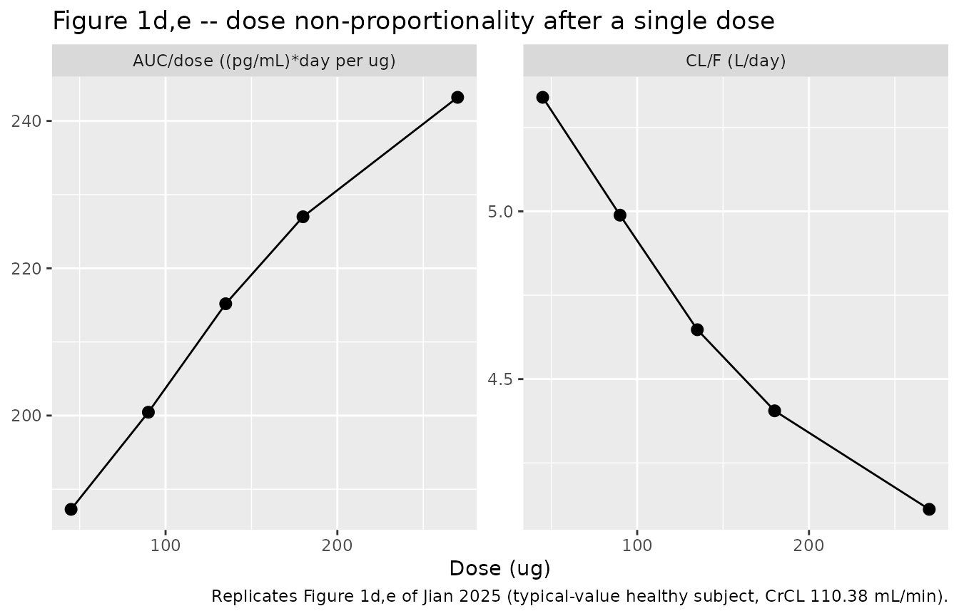


stopifnot(
  all(diff(np$auc_per_dose) > 0),  # AUC/dose increases with dose (Fig 1d)
  all(diff(np$clf_per_day)  < 0)   # CL/F decreases with dose (Fig 1e)
)
knitr::kable(np |> select(`Dose (ug)` = dose_ug,
                          `AUC/dose ((pg/mL)*day/ug)` = auc_per_dose,
                          `CL/F (L/day)` = clf_per_day),
             digits = 1,
             caption = "Saturable elimination: AUC/dose rises and CL/F falls across the studied dose range.")

Saturable elimination: AUC/dose rises and CL/F falls across the studied dose range.
Dose (ug)	AUC/dose ((pg/mL)*day/ug)	CL/F (L/day)
45	187.3	5.3
90	200.5	5.0
135	215.2	4.6
180	227.0	4.4
270	243.2	4.1

Figure 1c – exposure rises from week 1 to week 8 to week 48

The receptor-downregulation mechanism was added precisely because observed week-48 exposure exceeded week-8 exposure, which a classical TMDD model cannot produce (Jian 2025 Section 3.2 and Figure 1c).

interval_auc <- function(df) {
  df |>
    filter(!is.na(Cc)) |>
    group_by(arm, id) |>
    reframe(week = WEEKS_OBS,
            auctau = vapply(WEEKS_OBS, function(w)
              auc_window(time, Cc, (w - 1) * 168, w * 168), numeric(1))) |>
    mutate(auc_per_dose = auctau / 180 / 24 * 1000)
}

wk <- interval_auc(sim_multi)

wk |>
  filter(arm %in% c("Healthy, CrCL 110", "CHB, CrCL 110")) |>
  mutate(week = factor(week, levels = WEEKS_OBS, labels = paste("Week", WEEKS_OBS))) |>
  ggplot(aes(week, auc_per_dose, fill = arm)) +
  geom_boxplot(outlier.size = 0.4, alpha = 0.75) +
  labs(x = NULL, y = "AUCtau/dose ((pg/mL)*day per ug)", fill = NULL,
       title = "Figure 1c -- dosing-interval exposure at weeks 1, 8 and 48",
       caption = "Replicates Figure 1c of Jian 2025 (180 ug weekly).")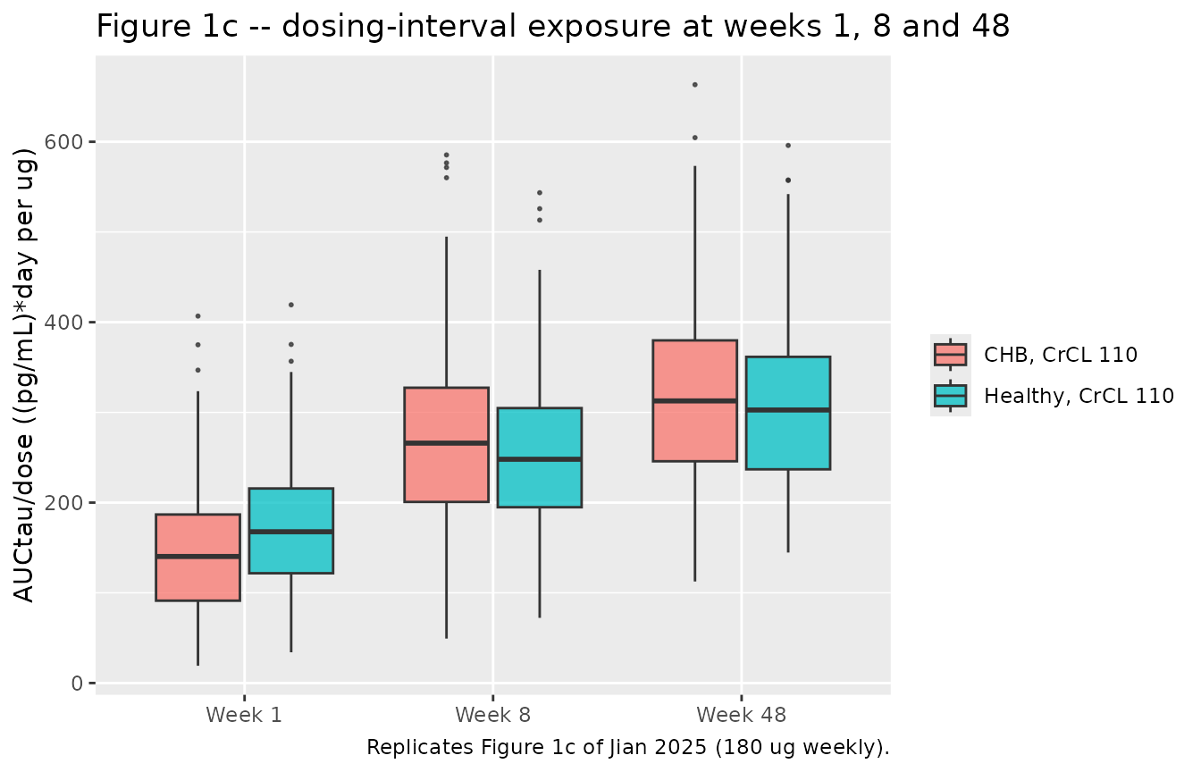


wk_typ <- interval_auc(simz_multi) |>
  filter(arm %in% c("Healthy, CrCL 110", "CHB, CrCL 110")) |>
  select(arm, week, auctau, auc_per_dose)

# Paper's claim: exposure increases monotonically week 1 -> 8 -> 48.
stopifnot(
  wk_typ |> group_by(arm) |> arrange(week, .by_group = TRUE) |>
    summarise(ok = all(diff(auctau) > 0), .groups = "drop") |> pull(ok) |> all()
)
knitr::kable(wk_typ |> tidyr::pivot_wider(id_cols = arm, names_from = week,
                                          values_from = auctau,
                                          names_prefix = "Week ") |>
               rename("Arm" = arm),
             digits = 0,
             caption = "Typical-value AUCtau (ug*h/L) per dosing interval. Exposure rises as receptor synthesis decays.")

Typical-value AUCtau (ug*h/L) per dosing interval. Exposure rises as receptor synthesis decays.
Arm	Week 1	Week 8	Week 48
CHB, CrCL 110	574	1132	1294
Healthy, CrCL 110	807	1134	1294

Figure 5e-h – health status at first dose and at steady state

Jian 2025 reports that the slower CHB absorption lowers both Cmax and AUC after the first dose (Figure 5e,f) but that, by steady state, receptor downregulation has made elimination essentially linear so the steady-state AUC is comparable between the two populations, with healthy subjects retaining a higher Cmax and larger peak-to-trough fluctuation (Figure 5g,h).

hs <- c("Healthy, CrCL 110", "CHB, CrCL 110")

simz_multi |>
  filter(!is.na(Cc), arm %in% hs, time >= 47 * 168) |>
  mutate(time_d = (time - 47 * 168) / 24) |>
  ggplot(aes(time_d, Cc, colour = arm)) +
  geom_line(linewidth = 0.9) +
  labs(x = "Time within the week-48 dosing interval (days)", y = "Cc (ug/L)", colour = NULL,
       title = "Figure 5g -- steady-state (week 48) concentration-time profile",
       caption = "Replicates Figure 5g of Jian 2025 (180 ug weekly, typical-value subject).")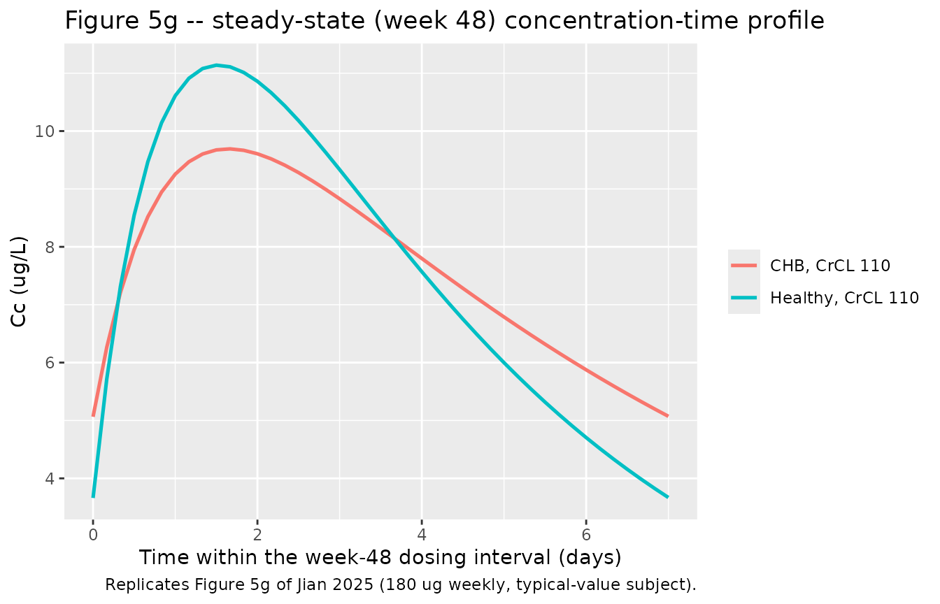


ss <- simz_multi |>
  filter(!is.na(Cc), arm %in% hs, time >= 47 * 168) |>
  group_by(arm) |>
  summarise(auctau = auc_window(time, Cc, 47 * 168, 48 * 168),
            cmax = max(Cc), ctrough = min(Cc), .groups = "drop") |>
  mutate(fluctuation = cmax / ctrough)

fd <- simz_single |>
  filter(!is.na(Cc), arm %in% c("Healthy 180 ug", "CHB 180 ug")) |>
  group_by(arm) |>
  summarise(auc = auc_window(time, Cc, 0, 720), cmax = max(Cc), .groups = "drop")

cl_typ  <- exp(unname(theta[["lcl"]]))
dose_cl <- 180 / cl_typ

# (a) First dose: healthy > CHB on BOTH Cmax and AUC (Figure 5e,f).
stopifnot(
  fd$cmax[fd$arm == "Healthy 180 ug"] > fd$cmax[fd$arm == "CHB 180 ug"],
  fd$auc [fd$arm == "Healthy 180 ug"] > fd$auc [fd$arm == "CHB 180 ug"]
)
# (b) Steady state: AUCtau comparable between populations (within 1%).
stopifnot(abs(diff(ss$auctau)) / mean(ss$auctau) < 0.01)
# (c) Steady state: elimination is essentially linear, so AUCtau ~ Dose/CL.
stopifnot(all(abs(ss$auctau / dose_cl - 1) < 0.05))
# (d) Healthy retains the higher Cmax and the larger fluctuation.
stopifnot(
  ss$cmax[ss$arm == "Healthy, CrCL 110"] > ss$cmax[ss$arm == "CHB, CrCL 110"],
  ss$fluctuation[ss$arm == "Healthy, CrCL 110"] > ss$fluctuation[ss$arm == "CHB, CrCL 110"]
)

bind_rows(
  fd |> transmute(Phase = "First dose", Arm = arm, `AUC (ug*h/L)` = auc,
                  `Cmax (ug/L)` = cmax, `Peak/trough` = NA_real_),
  ss |> transmute(Phase = "Steady state (week 48)", Arm = arm,
                  `AUC (ug*h/L)` = auctau, `Cmax (ug/L)` = cmax,
                  `Peak/trough` = fluctuation)
) |>
  knitr::kable(digits = 2,
               caption = sprintf(paste("Health status at first dose vs steady state (typical value, 180 ug).",
                                       "Steady-state Dose/CL = %.0f ug*h/L."), dose_cl))

Health status at first dose vs steady state (typical value, 180 ug). Steady-state Dose/CL = 1324 ug*h/L.
Phase	Arm	AUC (ug*h/L)	Cmax (ug/L)	Peak/trough
First dose	CHB 180 ug	888.74	4.68	NA
First dose	Healthy 180 ug	980.61	7.60	NA
Steady state (week 48)	CHB, CrCL 110	1294.06	9.69	1.91
Steady state (week 48)	Healthy, CrCL 110	1293.83	11.14	3.04

The steady-state AUC values are identical to three significant figures because health status acts only on ka, and by week 48 the residual receptor pool is too small for the saturable route to matter – exactly the mechanism Jian 2025 invokes in the Discussion (“the total elimination of Pegbing at steady state primarily relied on linear clearance … comparable steady-state AUCs of Pegbing were estimated between CHB patients and healthy subjects”).

# Quantify that claim: fraction of total elimination flowing through the
# saturable (TMDD) route, at week 1 vs week 48, for the typical CHB subject.
kint_t <- exp(unname(theta[["lkint"]]))
vc_t   <- exp(unname(theta[["lvc"]]))

frac_tmdd <- simz_multi |>
  filter(!is.na(Cc), arm == "CHB, CrCL 110") |>
  mutate(week = cut(time, breaks = c(-1, 168, 8 * 168, 48 * 168),
                    labels = c("Week 1", "Week 8", "Week 48")),
         bound = Cc - cfree,
         rate_tmdd = kint_t * bound * vc_t,
         rate_lin  = cl_typ * cfree) |>
  filter(!is.na(week)) |>
  group_by(week) |>
  summarise(`TMDD share of elimination` = sum(rate_tmdd) / sum(rate_tmdd + rate_lin),
            .groups = "drop")

stopifnot(
  frac_tmdd$`TMDD share of elimination`[frac_tmdd$week == "Week 1"] >
    frac_tmdd$`TMDD share of elimination`[frac_tmdd$week == "Week 48"]
)
knitr::kable(frac_tmdd, digits = 3,
             caption = "The saturable elimination route fades as the receptor pool is downregulated.")

The saturable elimination route fades as the receptor pool is downregulated.
week	TMDD share of elimination
Week 1	0.628
Week 8	0.326
Week 48	0.050

Figure 5a-d – creatinine clearance

Jian 2025 reports that CrCL differences are negligible after the first dose but become visible at steady state (Figure 5a-d), and that the effect nevertheless fails the 80-120% clinical-relevance band.

crcl_arms <- c("CHB, CrCL 91 (10th pctile)", "CHB, CrCL 110", "CHB, CrCL 152 (90th pctile)")

sim_multi |>
  filter(!is.na(Cc), arm %in% crcl_arms, time >= 47 * 168) |>
  mutate(time_d = (time - 47 * 168) / 24) |>
  group_by(arm, time_d) |>
  summarise(Q05 = quantile(Cc, 0.05), Q50 = median(Cc), Q95 = quantile(Cc, 0.95),
            .groups = "drop") |>
  ggplot(aes(time_d, Q50, colour = arm, fill = arm)) +
  geom_ribbon(aes(ymin = Q05, ymax = Q95), alpha = 0.15, colour = NA) +
  geom_line(linewidth = 0.9) +
  labs(x = "Time within the week-48 dosing interval (days)", y = "Cc (ug/L)",
       colour = NULL, fill = NULL,
       title = "Figure 5c -- steady-state exposure by creatinine clearance",
       caption = "Replicates Figure 5c of Jian 2025 (CHB, 180 ug weekly; median and 90% prediction interval).")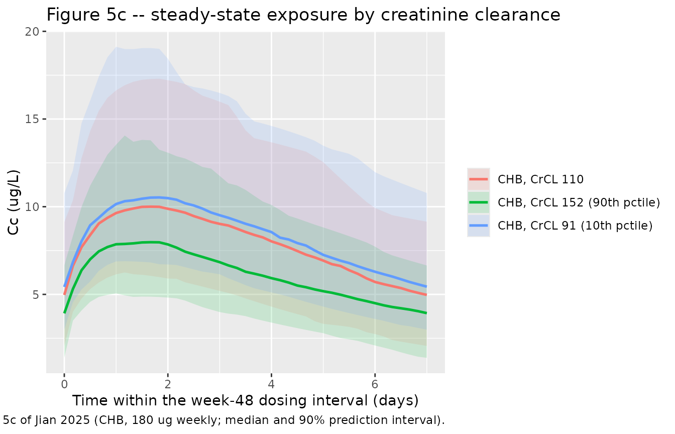


crcl_ss <- simz_multi |>
  filter(!is.na(Cc), arm %in% crcl_arms, time >= 47 * 168) |>
  group_by(arm, CRCL) |>
  summarise(auctau = auc_window(time, Cc, 47 * 168, 48 * 168), .groups = "drop") |>
  arrange(CRCL) |>
  mutate(ratio_vs_ref = auctau / auctau[which.min(abs(CRCL - CRCL_REF))])

# Higher CrCL -> higher clearance -> lower steady-state exposure.
stopifnot(all(diff(crcl_ss$auctau) < 0))
# At steady state elimination is linear, so the AUC ratio should be the
# reciprocal of the published CL ratio.
published_cl_ratio <- c(0.904, 1.0, 1.21)
stopifnot(max(abs(crcl_ss$ratio_vs_ref - 1 / published_cl_ratio)) < 0.02)

knitr::kable(crcl_ss |> rename("Arm" = arm, "CrCL (mL/min)" = CRCL,
                               "AUCtau (ug*h/L)" = auctau,
                               "AUC ratio vs reference" = ratio_vs_ref),
             digits = 3,
             caption = "Steady-state exposure vs CrCL; the AUC ratio is the reciprocal of the published CL ratio (0.904 / 1.21).")

Steady-state exposure vs CrCL; the AUC ratio is the reciprocal of the published CL ratio (0.904 / 1.21).
Arm	CrCL (mL/min)	AUCtau (ug*h/L)	AUC ratio vs reference
CHB, CrCL 91 (10th pctile)	91.332	1427.483	1.103
CHB, CrCL 110	110.380	1294.063	1.000
CHB, CrCL 152 (90th pctile)	152.047	1075.907	0.831

PKNCA validation

NCA is run on the single-dose arms. Following the paper’s bioanalytical method, each subject’s profile is truncated at the last point at or above the ELISA LLOQ of 300 pg/mL (= 0.3 ug/L); this both matches what the assay could see and keeps the terminal-slope fit out of the solver-noise tail.

LLOQ <- 0.3

sim_nca <- sim_single |>
  filter(!is.na(Cc)) |>
  group_by(id) |>
  filter(time <= max(time[Cc >= LLOQ])) |>
  ungroup() |>
  select(id, time, Cc, arm, dose_ug)

# Guarantee a time-zero row per subject (extravascular pre-dose Cc = 0).
sim_nca <- bind_rows(
  sim_nca,
  sim_nca |> distinct(id, arm, dose_ug) |> mutate(time = 0, Cc = 0)
) |>
  distinct(id, arm, time, .keep_all = TRUE) |>
  arrange(id, time)

conc_obj <- PKNCA::PKNCAconc(as.data.frame(sim_nca), Cc ~ time | arm + id)

dose_df <- ev_single |>
  filter(evid == 1) |>
  select(id, time, amt, arm)
dose_obj <- PKNCA::PKNCAdose(as.data.frame(dose_df), amt ~ time | arm + id)

intervals <- data.frame(
  start = 0, end = Inf,
  cmax = TRUE, tmax = TRUE, auclast = TRUE, aucinf.obs = TRUE,
  half.life = TRUE, cl.obs = TRUE
)

nca_res <- PKNCA::pk.nca(PKNCA::PKNCAdata(conc_obj, dose_obj, intervals = intervals))

nca_summary <- as.data.frame(nca_res) |>
  filter(PPTESTCD %in% c("cmax", "tmax", "aucinf.obs", "half.life", "cl.obs")) |>
  group_by(arm, PPTESTCD) |>
  summarise(median = median(PPORRES, na.rm = TRUE), .groups = "drop") |>
  tidyr::pivot_wider(names_from = PPTESTCD, values_from = median)

nca_summary |>
  mutate(half.life_d = half.life / 24) |>
  rename("Arm" = arm, "Cmax (ug/L)" = cmax, "Tmax (h)" = tmax,
         "AUCinf (ug*h/L)" = aucinf.obs, "t1/2 (h)" = half.life,
         "t1/2 (days)" = half.life_d, "CL/F (L/h)" = cl.obs) |>
  knitr::kable(digits = 2,
               caption = "Median simulated single-dose NCA by arm (100 virtual subjects per arm).")

Median simulated single-dose NCA by arm (100 virtual subjects per arm).
Arm	AUCinf (ug*h/L)	CL/F (L/h)	Cmax (ug/L)	t1/2 (h)	Tmax (h)	t1/2 (days)
CHB 180 ug	842.72	0.21	4.30	106.77	42	4.45
Healthy 135 ug	703.15	0.19	5.50	67.61	34	2.82
Healthy 180 ug	982.99	0.18	7.08	68.33	38	2.85
Healthy 270 ug	1691.72	0.16	12.43	65.31	42	2.72
Healthy 45 ug	185.14	0.24	1.26	68.70	30	2.86
Healthy 90 ug	436.78	0.21	3.25	70.56	32	2.94

Comparison against published NCA

Jian 2025 does not publish an NCA table; the only NCA-comparable number in the paper is the post-hoc elimination half-life quoted in the Discussion (“the elimination half-life of Pegbing is about 7 days”). It is compared below.

published <- tibble::tribble(
  ~arm,              ~half.life,
  "Healthy 180 ug",  7 * 24,
  "CHB 180 ug",      7 * 24
)

cmp <- nlmixr2lib::ncaComparisonTable(
  simulated     = nca_res,
  reference     = published,
  by            = "arm",
  params        = "half.life",
  units         = c(half.life = "h"),
  tolerance_pct = 20
)

knitr::kable(cmp,
             caption = "Simulated vs published terminal half-life. * differs from the reference by >20%.")

Simulated vs published terminal half-life. * differs from the reference by >20%.
NCA parameter	arm	Reference	Simulated	% diff
t½ (h)	Healthy 180 ug	168	68.3	-59.3%*
t½ (h)	CHB 180 ug	168	107	-36.4%*

This row is starred, and the discrepancy is real rather than an artefact of the simulation. With ka (0.0101 1/h healthy, 0.00601 1/h CHB) far smaller than kel = CL/V (0.0461 1/h), the model is firmly flip-flop: the terminal slope is set by absorption, giving log(2)/ka = 68.6 h (2.9 days) in healthy subjects and 115 h (4.8 days) in CHB patients. TMDD only steepens the true terminal phase further. No combination of the published Table 2 estimates yields a 7-day terminal half-life; see “Assumptions and deviations” below. No parameter has been adjusted to close the gap.

ka_h <- ka_healthy; ka_c <- ka_chb
kel  <- cl_typ / exp(unname(theta[["lvc"]]))
stopifnot(ka_h < kel, ka_c < kel)   # flip-flop confirmed
tibble::tibble(
  Quantity = c("ka healthy (1/h)", "ka CHB (1/h)", "kel = CL/V (1/h)",
               "log(2)/ka healthy (days)", "log(2)/ka CHB (days)",
               "log(2)/kel (days)"),
  Value = c(ka_h, ka_c, kel, log(2) / ka_h / 24, log(2) / ka_c / 24, log(2) / kel / 24)
) |>
  knitr::kable(digits = 4,
               caption = "Absorption is rate-limiting, so the terminal slope reflects ka, not CL/V.")

Absorption is rate-limiting, so the terminal slope reflects ka, not CL/V.
Quantity	Value
ka healthy (1/h)	0.0101
ka CHB (1/h)	0.0060
kel = CL/V (1/h)	0.0461
log(2)/ka healthy (days)	2.8595
log(2)/ka CHB (days)	4.8059
log(2)/kel (days)	0.6265

Assumptions and deviations

Equation 11 sign (corrected from the control stream). As typeset, Jian 2025 Eq. 11 reads ksyn = kdeg * R0 * exp(kR * t) with no minus sign (confirmed against the published PDF; minus signs render correctly in Eqs. 5, 6 and 9 of the same paper). The Data S2 final-model control stream settles it directly – it codes KSYN = REC0*KDEG*EXP(-THETA(9)*TIME) – so the executed model decays and the typeset equation is simply missing its minus. The model implements the decay form. The same conclusion follows four more ways from the paper’s own content, independent of the supplement:
1. the sentence introducing Eq. 11 – “the synthesis rate of receptors decreases exponentially from the beginning of treatment”; (ii) the Figure 2 caption – “kR, exponential decrease rate of IFN receptor”;
2. the Discussion’s “decrease by half after 14.5 weeks”, which reproduces log(2)/0.0068 per day = 14.56 weeks only under decay; and (iv) the Discussion’s “reduced to approximately 10% of baseline” after 48 weeks, which reproduces exp(-0.0068 * 336) = 0.102 only under decay. With the printed + sign the receptor pool would grow to roughly 9.8x baseline by week 48, inverting the very observation (Figure 1c) the mechanism was introduced to explain.
Published terminal half-life is not reproducible from Table 2. The Discussion states “the elimination half-life of Pegbing is about 7 days”; the Table 2 parameter set implies 2.9 days (healthy) to 4.8 days (CHB), as shown above. The parameters are used as published.
Table 2 back-transform footnote (settled by $OMEGA / $SIGMA). The abbreviations footnote defines the reported percentages as SQRT(omega^2 - 1) and SQRT(sigma^2 - 1), which is impossible for these estimates (it would need omega^2 > 1). Two readings were plausible from the main text alone: the log-normal CV SQRT(exp(omega^2) - 1), or the log-scale SD SQRT(omega^2). The Data S2 $OMEGA block decides it – and the two readings differ by up to 7 percentage points, so this is not a cosmetic choice:

Parameter $OMEGA variance 100*sqrt(var) 100*sqrt(exp(var)-1) Table 2

CL/F 0.118 34.4 35.4 34.4

V/F 0.232 48.2 51.1 48.2

ka 0.197 44.4 46.7 44.4

kint 0.272 52.2 55.9 52.2

100*sqrt(variance) reproduces every printed digit; the log-normal CV matches none. The $SIGMA variances (0.037 and 15100 pg^2/mL2) back out to 19.2% and 123 pg/mL on the same scale. The variances are therefore taken from $OMEGA / $SIGMA verbatim, not back-transformed. The footnote’s label “CI, confidence interval” attached to that formula is a further slip for “CV”.
CrCL effect is linear, not exponential. The Jian 2025 Table 2 row label prints CL x exp(theta x (CrCL-110.38)), but the executed Data S2 control stream codes the linear relation CLB_CLCR=(1+THETA(11)*(B_CLCR-110.38)) – Equation 1 of Methods Section 2.3, the PsN stepwise-covariate-model linear form. The model follows the control stream. Over the observed CrCL range (67.6-187.0 mL/min, Table 1) the two forms differ by up to about 6% in CL, so the choice is visible but not dramatic. The control stream also shows the covariate is baseline CrCL (B_CLCR), not the time-varying CLCR column that the dataset also carries.
Covariate screening path. Table S1 (Data S1) records the full stepwise path: forward inclusion added health status on ka (dOFV -15.84), CrCL on CL (-7.43) and body weight on V (-5.77); backward elimination then dropped weight on V (+5.74, below the 6.63 threshold) while retaining CrCL on CL (+10.01) and health status on ka (+15.77). This confirms the two-covariate final model implemented here.
Table 2 bootstrap-median typo for R0. The final-model bootstrap median for R0 prints as 0.0328, ten-fold below the 0.328 point estimate and outside its own bootstrap 95% CI (0.255-0.474). The point estimate is used.
ka units in the Discussion. The Discussion compares “a higher absorption rate constant (0.010/day v.s. 0.00583/day)”, but Table 2 labels ka as /h in both the base and final model blocks (and reserves 1/day for kR, showing the units were tracked per row). The /h reading is used: at 0.0101/day the absorption half-life would be 69 days, which is incompatible with the 17-day Phase I sampling window and with the observed Tmax.
Bioavailability. Eq. 5 sets Xa(0) = Dose with no separate F term, so F = 1 and both CL/F and V/F are apparent. Figure 2 draws an F but it is not identifiable and is not estimated.
Observed analyte. The ELISA quantifies total drug, and Jian 2025 integrates Drugtol; the model therefore reports Cc = Ctol. Free concentration is available as the derived variable cfree. The paper does not state the total-vs-free assay specificity explicitly.
Receptor state units. total_target carries a drug-equivalent concentration (ug/L), not an amount: Eq. 9 is written on the concentration scale and Table 2 reports R0 in ug/L, even though the symbol glossary loosely calls Rtol an “amount”.
kint < kdeg stabilises the receptor pool transiently. With the published kint = 0.0827/h and the Besremi-fixed kdeg = 0.544/h, the -(kint - kdeg) * bound term of Eq. 9 is positive while drug is bound, so total receptor rises above R0 early in treatment before the ksyn decay takes over (it falls to ~63% of R0 by week 48 in the typical subject, while the synthesis rate falls to ~10%). This is the standard Gibiansky QSS/QE Rtot equation evaluated at the published constants, not a transcription choice; the Discussion’s “reduced to approximately 10% of baseline” describes the synthesis rate / drug-free equivalent baseline.
Covariate polarity. The canonical register column is DIS_HEALTHY (1 = healthy), while Jian 2025 uses healthy as the reference and reports the effect on the CHB arm. The model evaluates the complement (1 - DIS_HEALTHY) so the published (1 + theta) form is reproduced exactly.
Base model excluded. Jian 2025 Table 2 also reports a base (no-covariate) model. Per the library’s replicate-the-authors policy, only the final model is packaged; the base-model estimates are recorded in the source-trace notes only.
Body weight is not in the final model. The Abstract claims “body weight affected the volume of distribution”, but the Discussion states weight was dropped in backward elimination and Table 2’s final model has no weight term. Weight is recorded in covariatesDataExcluded, not covariateData. The Data S2 control stream corroborates this in a third way: it still contains the vestigial line TVV = VCOV*TVV from the PsN stepwise-covariate-model template, but VCOV is never assigned anywhere in $PK – the weight-on-V block was deleted during backward elimination and only its consumer was left behind. The reported V/F equals THETA(2) exactly (2.95 L), so the executed model carried no covariate on V. This model therefore applies none.
Table 1 validation-cohort sex percentages are transposed (printed as Male 84 (27.0%) / Female 31 (73.0%), but 84/115 = 73.0%). This affects only the held-out external-validation cohort description, not the model.
Supplement. Data S1-S3 were retrieved from the Europe PMC supplementaryFiles endpoint for PMC12706394 and are the source of the three corrections above. Data S3 (PSP4-14-2014-s003.csv) is a single-subject example dataset, not the analysis dataset, so no subject-level distribution could be recovered from it; the virtual cohorts below use the Table 1 summaries instead.
Virtual cohorts. Covariates are fixed per arm at the values Jian 2025 uses for its own covariate simulations (Section 2.4), with between-subject spread supplied by the estimated IIV. Cohorts are 100 (single-dose) or 120 (multiple-dose) subjects per arm.

Parameter	`$OMEGA` variance	`100*sqrt(var)`	`100*sqrt(exp(var)-1)`	Table 2
CL/F	0.118	34.4	35.4	34.4
V/F	0.232	48.2	51.1	48.2
ka	0.197	44.4	46.7	44.4
kint	0.272	52.2	55.9	52.2