Ropeginterferon alfa-2b (Qin 2025)
Source:vignettes/articles/Qin_2025_ropeginterferon.Rmd
Qin_2025_ropeginterferon.RmdModel and source
- Citation: Qin A, Shimoda K, Suo S, Fu R, Kirito K, Wu D, Liao J, Chen H, Wu L, Su X, Gao Y, Sato T, Li Y, Zhang J, Shen W, Wang W, Zhang L, Jin J, Komatsu N. Population pharmacokinetics-pharmacodynamics and exposure-response of ropeginterferon alfa-2b in Chinese and Japanese patients with polycythemia vera. Pharmacol Res Perspect. 2025;13(3):e70109. doi:10.1002/prp2.70109.
- Article (open access): https://doi.org/10.1002/prp2.70109
- Supporting Information (Figures S1-S7 and Table S1, one DOCX):
available from the article landing page and from Europe PMC as
PRP2-13-e70109-s001.docxunder PMC12046122.
Qin 2025 is a single paper carrying eleven separately fitted models. All eleven are packaged here.
| Model |
modellib() name |
Source |
|---|---|---|
| Population PK (quasi-equilibrium TMDD) | Qin_2025_ropeginterferon |
Table 2, Figure 1A |
| PK-PD, hematocrit | Qin_2025_ropeginterferon_hct |
Table 3 (HCT), Figure 1B |
| PK-PD, platelet count | Qin_2025_ropeginterferon_plt |
Table 3 (PLT), Figure 1C |
| PK-PD, white blood cell count | Qin_2025_ropeginterferon_wbc |
Table 3 (WBC), Figure 1C |
| E-R, complete hematologic response at week 24 | Qin_2025_ropeginterferon_chr_week24 |
Table 4, Equation (3) |
| E-R, complete hematologic response at week 52 | Qin_2025_ropeginterferon_chr_week52 |
Table 4, Equation (4) |
| E-R, JAK2 V617F change at week 24 | Qin_2025_ropeginterferon_jak2_week24 |
Table 4, Equation (5) |
| E-R, JAK2 V617F change at week 52 | Qin_2025_ropeginterferon_jak2_week52 |
Table 4, Equation (5) |
| E-R, titration-phase ALT increase | Qin_2025_ropeginterferon_alt_increase |
Results 3.4, Equation (3) |
| E-R, titration-phase AST increase | Qin_2025_ropeginterferon_ast_increase |
Results 3.4, Equation (3) |
| E-R, maintenance-phase anemia | Qin_2025_ropeginterferon_anemia |
Results 3.4, Equation (3), Figure 5C-D |
mod_pk   <- rxode2::rxode(readModelDb("Qin_2025_ropeginterferon"))
mod_hct  <- rxode2::rxode(readModelDb("Qin_2025_ropeginterferon_hct"))
mod_plt  <- rxode2::rxode(readModelDb("Qin_2025_ropeginterferon_plt"))
mod_wbc  <- rxode2::rxode(readModelDb("Qin_2025_ropeginterferon_wbc"))
mod_chr24 <- rxode2::rxode(readModelDb("Qin_2025_ropeginterferon_chr_week24"))
mod_chr52 <- rxode2::rxode(readModelDb("Qin_2025_ropeginterferon_chr_week52"))
mod_jak24 <- rxode2::rxode(readModelDb("Qin_2025_ropeginterferon_jak2_week24"))
mod_jak52 <- rxode2::rxode(readModelDb("Qin_2025_ropeginterferon_jak2_week52"))
mod_alt  <- rxode2::rxode(readModelDb("Qin_2025_ropeginterferon_alt_increase"))
mod_ast  <- rxode2::rxode(readModelDb("Qin_2025_ropeginterferon_ast_increase"))
mod_anemia <- rxode2::rxode(readModelDb("Qin_2025_ropeginterferon_anemia"))
Population
Ropeginterferon alfa-2b (ropeg) is a mono-PEGylated interferon alfa-2b approved for polycythaemia vera (PV) by the EMA in 2019, the FDA in 2021, and in Japan and China thereafter. The population PK analysis pools four studies and 126 participants; the PK-PD and exposure-response analyses use only the 78 PV patients.
| Study | n | Population | Regimen |
|---|---|---|---|
| A17-101 (CTR20190451) | 18 | Healthy Chinese adults | Single SC dose, 90-270 ug |
| A17-102 (NCT03546465) | 30 | Healthy Japanese (and Caucasian) adults | Single SC dose, 100-300 ug |
| A19-201 (NCT04182100) | 29 | Japanese patients with PV | SC q2w, slow titration: start 100 ug (50 ug if on prior cytoreductive therapy), +50 ug q2w to a 500 ug maximum |
| A20-202 (NCT05485948) | 49 | Chinese patients with PV, hydroxyurea-resistant or -intolerant | SC q2w, fast titration: 250 ug at week 0, 350 ug at week 2, 500 ug from week 4 |
Pooled baseline characteristics (Qin 2025 Table 1, “Overall” column, n = 126): median age 43.5 years (21.0-72.0), median weight 62.8 kg (43.6-91.0), median BMI 23.1 kg/m^2 (17.4-32.2), 47/126 (37.3%) female. Median baseline JAK2 V617F allele burden is 77.8% in A19-201 and 61.2% in A20-202; the healthy cohorts are 0% by construction.
The pooled BMI median of 23.1 kg/m^2 is load-bearing: it is the centring constant of the only covariate in the model.
pk_pop <- mod_pk$meta$population
tibble::tibble(
  Field = names(pk_pop),
  Value = vapply(pk_pop, function(x) paste(format(x), collapse = "; "), character(1))
) |>
knitr::kable(caption = "Population metadata carried by the population PK model.")| Field | Value |
|---|---|
| species | human |
| n_subjects | 126 |
| n_studies | 4 |
| n_observations | not reported as a record count; PK sampling was pre-dose and 1, 3, 6, 9, 12, 24, 36, 48, 72, 96, 120, 144, 168, 192, 240, 288, 336, 504 and 672 h post-dose in both phase I studies, and weeks 0 and 28 (A19-201) or weeks 0 and 12 (A20-202) pre-dose plus 48, 96 and 168 h post-dose with trough concentrations at every visit in the phase II studies |
| age_range | median 43.5 years, range 21.0-72.0 pooled (Qin 2025 Table 1, Overall); healthy phase I median 27.0-30.0 years, PV phase II median 54.0-56.0 years |
| weight_range | median 62.8 kg, range 43.6-91.0 (Qin 2025 Table 1, Overall) |
| bmi_range | median 23.1 kg/m^2, range 17.4-32.2 (Qin 2025 Table 1, Overall); this median is the centring value of the clearance covariate model |
| sex_female_pct | 37.3 |
| race_ethnicity | Chinese (A17-101 n = 18 healthy; A20-202 n = 49 PV) and Japanese (A19-201 n = 29 PV); A17-102 enrolled 30 healthy Japanese and Caucasian participants. Qin 2025 Methods 2.1: ‘Only participants from Japan and China who were administered ropeg were included in the analyses.’ |
| disease_state | 48 healthy volunteers and 78 patients with polycythaemia vera. All A20-202 patients and all but two A19-201 patients carried the JAK2 V617F driver mutation; A20-202 enrolled patients resistant to or intolerant of hydroxyurea. Baseline JAK2 V617F allele burden median 77.8% (A19-201) and 61.2% (A20-202) |
| dose_range | phase I single subcutaneous doses of 90-270 ug (A17-101) and 100-300 ug (A17-102); phase II subcutaneous doses every 2 weeks, A19-201 starting at 100 ug (or 50 ug on prior cytoreductive therapy) titrated in 50 ug steps to a 500 ug maximum (slow titration) and A20-202 starting at 250 ug with titration to 350 ug at week 2 and 500 ug from week 4 (fast titration) |
| regions | China (A17-101, A20-202) and Japan (A17-102, A19-201); A17-102 also enrolled Caucasian participants who were excluded from these analyses |
| trial_registration | A17-102 NCT03546465; A19-201 NCT04182100; A20-202 NCT05485948; A17-101 CTR20190451 (chinadrugtrials.org.cn) |
| notes | Ropeginterferon alfa-2b is approved for polycythaemia vera by the EMA (2019), the FDA (2021) and in Japan (2023) and China. The pooled analysis set spans a 10-fold single-dose range in healthy participants and up to 100 weeks of every-2-week dosing in patients, which is what identifies both the linear and the target-mediated elimination arms. All fixed and random effects were estimated with relative standard errors below 15% (Qin 2025 Results 3.2.1). |
Errata and unit reconciliation
The published rate constants are per DAY, not per hour
Qin 2025 Table 2 labels CL as L h-1 and
Ka, kint, kdeg and
kdec as h-1; Table 3 labels ktr,
kout,P and kout,W as h-1.
Those unit labels are wrong. Every one of those values is per
day. All ten packaged models therefore declare
units$time = "day" and use the printed values unchanged;
nothing is rescaled, only relabelled.
Four pieces of evidence, three of them mutually independent:
-
The paper contradicts its own tables. Methods 2.4.1
states that
kdecis “in day-1” and thatkoutis “in day-1”, while Tables 2 and 3 label the same two parametersh-1. -
Tmax. Read per day,
ka = 0.18andkel = CL/Vc = 0.753/3.29 = 0.2289giveTmax = ln(ka/kel)/(ka - kel) = 4.91 d = 118 h, and becauseka < kelthe terminal half-life is the flip-flopln(2)/ka = 92 h. Every single-dose panel of the supplementary PK visual predictive check (Figure S2, stratified by dose) peaks at 100-150 h after dose. Read per hour the same algebra givesTmax = 4.9 HOURS, which Figure S2 excludes outright. -
Cmax. A single 300 ug dose gives 29.6 ng/mL under
the day reading; the Figure S2
DOSEUG == 300panel peaks at 25-30 ng/mL. -
Cavg.
Dose/(CL*tau)for 500 ug q2w is 47.4 ng/mL under the day reading, and 19.9 ng/mL for the roughly 210 ug average dose of the slow-titration arm. Figure 3 puts the observed medianCavg,0-24Wat about 37.5 ng/mL (A20-202, fast titration) and about 20 ng/mL (A19-201, slow titration). Read per hour, 500 ug every 336 h gives 1.98 ng/mL, a 20-fold miss.
ka <- 0.18; cl <- 0.753; vc <- 3.29
day <- tibble::tibble(
  Quantity = c("Tmax (h)", "Terminal t1/2 (h)", "Cavg, 500 ug q2w (ng/mL)"),
  `Per-day reading` = c(
    24 * log(ka / (cl / vc)) / (ka - cl / vc),
    24 * log(2) / min(ka, cl / vc),
    500 / (cl * 14)),
  `Per-hour reading` = c(
    log(ka / (cl / vc)) / (ka - cl / vc),
    log(2) / min(ka, cl / vc),
    500 / (cl * 336)),
  `Observed (Figures S2, 3)` = c("100-150", "roughly 100", "about 37.5 at 500 ug q2w")
)
knitr::kable(day, digits = 2,
             caption = paste(
               "Only the per-day reading reproduces the published figures.",
               "The per-hour reading misses Tmax by a factor of 24 and Cavg by",
"a factor of 20."))| Quantity | Per-day reading | Per-hour reading | Observed (Figures S2, 3) |
|---|---|---|---|
| Tmax (h) | 117.96 | 4.91 | 100-150 |
| Terminal t1/2 (h) | 92.42 | 3.85 | roughly 100 |
| Cavg, 500 ug q2w (ng/mL) | 47.43 | 1.98 | about 37.5 at 500 ug q2w |
# The day reading must land inside the Figure S2 Tmax window and within 25% of
# the Figure 3 fast-titration Cavg; the hour reading must fail both.
tmax_day  <- 24 * log(ka / (cl / vc)) / (ka - cl / vc)
tmax_hour <- log(ka / (cl / vc)) / (ka - cl / vc)
stopifnot(
  tmax_day > 100, tmax_day < 150,
  tmax_hour < 10,
  abs(500 / (cl * 14) / 47.4 - 1) < 0.01,
  500 / (cl * 336) < 5
)
Absorption lag time and TSTART
Table 2 prints the absorption lag time as 0.62 labelled
(h) and TSTART as 7 labelled
(h). Both are carried here in days, for
internal consistency with the rate constants above. The choice is
numerically immaterial for the lag: Tmax is about 118 h, so moving the
lag between 0.62 h and 0.62 d shifts Cmax and AUC by well under 1%. It
is also immaterial for TSTART, because the binding capacity
it gates declines with a 27-day half-life
(ln(2)/0.0255 = 27.2 days), against which 7 h and 7 d are
indistinguishable.
Discussion-versus-Table conflict for platelets and white cells
Qin 2025’s Discussion restates the PK-PD parameters. For hematocrit it agrees with Table 3 to every printed digit (initial 45.9%, equilibrium 48.9%, Imax 59.2%, IC50 137 ng/mL). For platelets and white cells it does not:
| Endpoint | Quantity | Table 3 (used here) | Discussion |
|---|---|---|---|
| PLT | Initial | 477 | 463 |
| PLT | Equilibrium | 332 | 351 |
| PLT | IC50 | 72.4 | 61.9 |
| WBC | Initial | 11.4 | 12.1 |
| WBC | Equilibrium | 6.72 | 7.32 |
| WBC | IC50 | 152 | 124 |
Table 3 is used, because it is the designated
parameter-estimates table and carries relative standard errors, and
because the Discussion paragraph is demonstrably degraded: it labels the
platelet and white-cell quantities with the hematocrit
subscript H (kin,H, IC50,H) in all three
paragraphs. Where that subscript is correct, the two agree exactly.
Other reporting artefacts
-
Table 1 hematocrit, A20-202 column reads
45.7 [0.421, 64.1]: a median on the per-cent scale against a range that mixes the fraction and per-cent scales. The model’s hematocrit is a fraction (HCT0 = 0.459), which the A19-201 column (0.459 [0.356, 0.539]) and the Table 3 estimates confirm. -
Table 3 unit labels give
PLTss,PLT0,WBCssandWBC0as10^9 L-1 day-1, a rate. They are counts (10^9 L-1); onlykin, which the table does not report, carries theday-1. -
Covariance versus correlation. Table 3’s rows
“Covariance of IIV_X and IIV_IC50” are taken at face value as
covariances. All three are admissible as such (implied correlations
-0.873, -0.698, -0.500); the check is in the
ini()block of each PK-PD model.
Source trace
Every equation and every ini() value, with its source
location.
trace <- tibble::tribble(
  ~Component, ~Value, ~Source,
  "PK: depot -> serum, first-order with lag", "Ka, ALAG", "Figure 1A schematic",
  "PK: linear elimination on free drug", "CL/Vc", "Figure 1A schematic",
  "PK: quasi-equilibrium binding, complex internalised", "KD, kint, kdeg, ksyn", "Figure 1A schematic",
  "PK: ksyn = kdeg * Rtot, Rtot decays Rtot0 -> Rtot,SS after TSTART in patients", "kdec", "Methods 2.4.1 (prose)",
  "PK: continuous covariate model P_i = P_TV*(COV/COV_med)^theta", "e_bmi_cl", "Equation (1)",
  "Ka (1/day)", "0.18 (RSE 1.04%)", "Table 2",
  "Absorption lag (day)", "0.62 (RSE 0.421%)", "Table 2",
  "CL (L/day)", "0.753 (RSE 0.846%)", "Table 2",
  "Vc (L)", "3.29 (RSE 1.03%)", "Table 2",
  "Rtot0 (ng/mL)", "0.317 (RSE 0.904%)", "Table 2",
  "Rtot,SS (ng/mL)", "0.012 (RSE 0.997%)", "Table 2",
  "kint (1/day)", "0.0223 (RSE 0.88%)", "Table 2",
  "kdeg (1/day)", "0.51 (RSE 0.576%)", "Table 2",
  "KD (ng/mL)", "0.0662 (RSE 0.981%)", "Table 2",
  "kdec (1/day)", "0.0255 (RSE 0.892%)", "Table 2",
  "TSTART (day)", "7 (FIX)", "Table 2",
  "BMI effect on CL", "0.813 (RSE 9.39%)", "Table 2",
  "PK IIV (CV%): Ka/CL/Vc/Rtot0/kint", "69.9 / 35.3 / 94.6 / 272 / 125", "Table 2",
  "PK RUV: proportional / additive", "19.7% / 0.542 ng/mL", "Table 2",
  "HCT: dTransit/dt = kin*(1 - Imax*Cs/(IC50+Cs)) - ktr*Transit; dHCT/dt = ktr*(Transit - HCT)", "-", "Figure 1B (printed ODEs)",
  "HCT0 / HCTss / IC50 / Imax / ktr", "0.459 / 0.489 / 137 / 0.592 / 0.023", "Table 3 (HCT)",
  "HCT IIV (CV%) HCTss/IC50/ktr/HCT0; cov(HCTss,IC50)", "20 / 430 / 113 / 10.4; -0.298", "Table 3 (HCT)",
  "HCT RUV proportional", "4.09%", "Table 3 (HCT)",
  "PLT and WBC: dX/dt = kin*(1 - Imax*Cs/(IC50+Cs)) - kout*X", "-", "Figure 1C (printed ODEs)",
  "PLT0 / PLTss / IC50,P / Imax,P / kout,P", "477 / 332 / 72.4 / 1 (FIX) / 0.0299", "Table 3 (PLT)",
  "PLT IIV (CV%) PLTss/IC50/kout/PLT0; cov", "67.6 / 162 / 135 / 58.9; -0.486", "Table 3 (PLT)",
  "PLT RUV proportional", "12.1%", "Table 3 (PLT)",
  "WBC0 / WBCss / IC50,W / Imax,W / kout,W", "11.4 / 6.72 / 152 / 1 (FIX) / 0.0475", "Table 3 (WBC)",
  "WBC IIV (CV%) WBCss/IC50/kout/WBC0; cov", "47.4 / 102 / 131 / 62.5; -0.190", "Table 3 (WBC)",
  "WBC RUV proportional", "16%", "Table 3 (WBC)",
  "Hill coefficient tested and REJECTED for all three endpoints", "dOFV 0.016 (HCT), 5.654 (WBC), -35.489 (PLT)", "Results 3.2.2",
  "E-R logistic, linear: logit(P) = b0 + b1*Exposure + bT*X", "-", "Equation (3)",
  "E-R logistic, Emax: logit(P) = E0 + Emax*E/(EC50+E) + bT*X", "-", "Equation (4)",
  "E-R regression, linear: Y = b0 + b1*Exposure + bT*X", "-", "Equation (5)",
  "CHR week 24: b0 / b1", "-1.2614 (SE 0.6525) / 0.0411 (SE 0.0187)", "Table 4",
  "CHR week 52: E0 / Emax / EC50", "-7 (FIX) / 8.397 (SE 0.665) / 1.98 (SE 2.472)", "Table 4",
  "JAK2 week 24: b0 / b_exposure / b_weight", "30.728 (SE 11.601) / -0.51 (SE 0.141) / -0.435 (SE 0.169)", "Table 4",
  "JAK2 week 52: b0 / b_exposure", "-8.528 (SE 7.812) / -0.43 (SE 0.194)", "Table 4",
  "ALT increase: b0 / b_exposure", "-4.099 (SE 0.9843) / 0.1156 (SE 0.0399)", "Results 3.4 (running text)",
  "AST increase: b0 / b_exposure", "-4.75194 (SE 1.123) / 0.143564 (SE 0.0453)", "Results 3.4 (running text)",
  "Anemia: b0 / b_exposure / b_JAK2", "-6.95416 (SE 1.9606) / 0.056548 (SE 0.0258) / 0.041351 (SE 0.0175)", "Results 3.4 (running text)",
  "Anemia covariate scale: baseline JAK2 V617F in PER CENT", "77.8 [0.0210, 97.5] A19-201; 61.2 [4.70, 96.4] A20-202", "Table 1"
)
knitr::kable(trace, caption = "Source trace for every model equation and parameter.")| Component | Value | Source |
|---|---|---|
| PK: depot -> serum, first-order with lag | Ka, ALAG | Figure 1A schematic |
| PK: linear elimination on free drug | CL/Vc | Figure 1A schematic |
| PK: quasi-equilibrium binding, complex internalised | KD, kint, kdeg, ksyn | Figure 1A schematic |
| PK: ksyn = kdeg * Rtot, Rtot decays Rtot0 -> Rtot,SS after TSTART in patients | kdec | Methods 2.4.1 (prose) |
| PK: continuous covariate model P_i = P_TV*(COV/COV_med)^theta | e_bmi_cl | Equation (1) |
| Ka (1/day) | 0.18 (RSE 1.04%) | Table 2 |
| Absorption lag (day) | 0.62 (RSE 0.421%) | Table 2 |
| CL (L/day) | 0.753 (RSE 0.846%) | Table 2 |
| Vc (L) | 3.29 (RSE 1.03%) | Table 2 |
| Rtot0 (ng/mL) | 0.317 (RSE 0.904%) | Table 2 |
| Rtot,SS (ng/mL) | 0.012 (RSE 0.997%) | Table 2 |
| kint (1/day) | 0.0223 (RSE 0.88%) | Table 2 |
| kdeg (1/day) | 0.51 (RSE 0.576%) | Table 2 |
| KD (ng/mL) | 0.0662 (RSE 0.981%) | Table 2 |
| kdec (1/day) | 0.0255 (RSE 0.892%) | Table 2 |
| TSTART (day) | 7 (FIX) | Table 2 |
| BMI effect on CL | 0.813 (RSE 9.39%) | Table 2 |
| PK IIV (CV%): Ka/CL/Vc/Rtot0/kint | 69.9 / 35.3 / 94.6 / 272 / 125 | Table 2 |
| PK RUV: proportional / additive | 19.7% / 0.542 ng/mL | Table 2 |
| HCT: dTransit/dt = kin(1 - ImaxCs/(IC50+Cs)) - ktrTransit; dHCT/dt = ktr(Transit - HCT) | - | Figure 1B (printed ODEs) |
| HCT0 / HCTss / IC50 / Imax / ktr | 0.459 / 0.489 / 137 / 0.592 / 0.023 | Table 3 (HCT) |
| HCT IIV (CV%) HCTss/IC50/ktr/HCT0; cov(HCTss,IC50) | 20 / 430 / 113 / 10.4; -0.298 | Table 3 (HCT) |
| HCT RUV proportional | 4.09% | Table 3 (HCT) |
| PLT and WBC: dX/dt = kin(1 - ImaxCs/(IC50+Cs)) - kout*X | - | Figure 1C (printed ODEs) |
| PLT0 / PLTss / IC50,P / Imax,P / kout,P | 477 / 332 / 72.4 / 1 (FIX) / 0.0299 | Table 3 (PLT) |
| PLT IIV (CV%) PLTss/IC50/kout/PLT0; cov | 67.6 / 162 / 135 / 58.9; -0.486 | Table 3 (PLT) |
| PLT RUV proportional | 12.1% | Table 3 (PLT) |
| WBC0 / WBCss / IC50,W / Imax,W / kout,W | 11.4 / 6.72 / 152 / 1 (FIX) / 0.0475 | Table 3 (WBC) |
| WBC IIV (CV%) WBCss/IC50/kout/WBC0; cov | 47.4 / 102 / 131 / 62.5; -0.190 | Table 3 (WBC) |
| WBC RUV proportional | 16% | Table 3 (WBC) |
| Hill coefficient tested and REJECTED for all three endpoints | dOFV 0.016 (HCT), 5.654 (WBC), -35.489 (PLT) | Results 3.2.2 |
| E-R logistic, linear: logit(P) = b0 + b1Exposure + bTX | - | Equation (3) |
| E-R logistic, Emax: logit(P) = E0 + EmaxE/(EC50+E) + bTX | - | Equation (4) |
| E-R regression, linear: Y = b0 + b1Exposure + bTX | - | Equation (5) |
| CHR week 24: b0 / b1 | -1.2614 (SE 0.6525) / 0.0411 (SE 0.0187) | Table 4 |
| CHR week 52: E0 / Emax / EC50 | -7 (FIX) / 8.397 (SE 0.665) / 1.98 (SE 2.472) | Table 4 |
| JAK2 week 24: b0 / b_exposure / b_weight | 30.728 (SE 11.601) / -0.51 (SE 0.141) / -0.435 (SE 0.169) | Table 4 |
| JAK2 week 52: b0 / b_exposure | -8.528 (SE 7.812) / -0.43 (SE 0.194) | Table 4 |
| ALT increase: b0 / b_exposure | -4.099 (SE 0.9843) / 0.1156 (SE 0.0399) | Results 3.4 (running text) |
| AST increase: b0 / b_exposure | -4.75194 (SE 1.123) / 0.143564 (SE 0.0453) | Results 3.4 (running text) |
| Anemia: b0 / b_exposure / b_JAK2 | -6.95416 (SE 1.9606) / 0.056548 (SE 0.0258) / 0.041351 (SE 0.0175) | Results 3.4 (running text) |
| Anemia covariate scale: baseline JAK2 V617F in PER CENT | 77.8 [0.0210, 97.5] A19-201; 61.2 [4.70, 96.4] A20-202 | Table 1 |
Virtual cohort and simulation
Two cohorts of 150 participants each: a healthy phase I cohort for
the single-dose pharmacokinetics, and one polycythaemia
vera cohort that is put through both titration schedules.
DIS_HEALTHY is 1 for the healthy cohort and 0 for the PV
cohort, which is what switches the chronic target down-regulation on and
off.
Using a single PV cohort for both schedules, and re-seeding immediately before each solve so the two arms draw the same random effects, is not a convenience: it is what Qin 2025 did, and it is what makes the fast-versus-slow contrast interpretable. Results 3.2.3: “we simulated the PK-PD relationships for patients in the slow- and fast-dose titration regimens, and the difference between the two titration regimens was compared for each participant. This model can exclude the influence of interference factors, including inter-individual and inter-trial differences.” Two independently drawn cohorts would confound the schedule difference with the covariate and random-effect difference between them.
n_sub <- 150L

rxode2::rxSetSeed(20250501)
draw_cohort <- function(n, wt_med, wt_lo, wt_hi, bmi_med, bmi_lo, bmi_hi, healthy) {
  # Log-normal draws truncated to the published ranges; the SD is chosen so the
  # published range spans about +/- 2 SD on the log scale.
  rtrunc <- function(med, lo, hi) {
    s <- (log(hi) - log(lo)) / 4
    pmin(pmax(med * exp(stats::rnorm(n, 0, s)), lo), hi)
  }
  tibble::tibble(
    id = seq_len(n),
    WT = rtrunc(wt_med, wt_lo, wt_hi),
    BMI = rtrunc(bmi_med, bmi_lo, bmi_hi),
    DIS_HEALTHY = healthy
  )
}

coh_healthy <- draw_cohort(n_sub, 71.7, 51.4, 84.4, 25.5, 19.1, 29.5, 1)
# One PV cohort, put through both schedules. Weight and BMI are drawn to span
# the pooled A19-201 + A20-202 characteristics of Qin 2025 Table 1.
coh_pv <- draw_cohort(n_sub, 62.5, 43.6, 91.0, 22.9, 17.4, 32.2, 0)

summ <- function(d, lab) tibble::tibble(
  Cohort = lab,
  `Median WT (kg)` = stats::median(d$WT),
  `Median BMI (kg/m2)` = stats::median(d$BMI),
  DIS_HEALTHY = unique(d$DIS_HEALTHY))
dplyr::bind_rows(
  summ(coh_healthy, "Healthy, single 300 ug (phase I)"),
  summ(coh_pv, "Polycythaemia vera (both schedules)")) |>
knitr::kable(digits = 1, caption = "Simulated cohorts (150 participants each).")| Cohort | Median WT (kg) | Median BMI (kg/m2) | DIS_HEALTHY |
|---|---|---|---|
| Healthy, single 300 ug (phase I) | 72.4 | 25.7 | 1 |
| Polycythaemia vera (both schedules) | 62.7 | 22.3 | 0 |
# Fast titration (A20-202): 250 ug at week 0, 350 ug at week 2, 500 ug from
# week 4 (Qin 2025 Methods 2.1). Simulated to week 100 as in Figure 2.
n_dose  <- 50L
amt_fast <- c(250, 350, rep(500, n_dose - 2L))
# Slow titration (A19-201): start 100 ug, +50 ug every 2 weeks to a 500 ug
# maximum. This is the PROTOCOL-SPECIFIED schedule; see the note below the
# exposure table for why real A19-201 exposure was lower.
amt_slow <- pmin(100 + 50 * (seq_len(n_dose) - 1L), 500)
dose_times <- 14 * (seq_len(n_dose) - 1L)

build_ev <- function(coh, amt, times, obs) {
  dose <- tidyr::expand_grid(id = coh$id, k = seq_along(times)) |>
    dplyr::mutate(time = times[k], amt = amt[k], evid = 1L, cmt = "depot") |>
    dplyr::select(id, time, amt, evid, cmt)
  ob <- tidyr::expand_grid(id = coh$id, time = obs) |>
    dplyr::mutate(amt = NA_real_, evid = 0L, cmt = NA_character_)
  dplyr::bind_rows(dose, ob) |>
    dplyr::arrange(id, time, dplyr::desc(evid)) |>
    dplyr::left_join(coh, by = "id")
}
Single-dose pharmacokinetics (phase I)
rxode2::rxSetSeed(20250502)
obs_single <- sort(unique(c(seq(0, 30, by = 0.25), 0.62)))
ev_single <- build_ev(coh_healthy, 300, 0, obs_single)
sim_single <- rxode2::rxSolve(mod_pk, ev_single, returnType = "data.frame") |>
  dplyr::mutate(treatment = "300 ug single dose (healthy)")

sim_single |>
  dplyr::group_by(time) |>
  dplyr::summarise(med = stats::median(Cc),
                   lo = stats::quantile(Cc, 0.05),
                   hi = stats::quantile(Cc, 0.95), .groups = "drop") |>
  ggplot(aes(24 * time, med)) +
  geom_ribbon(aes(ymin = lo, ymax = hi), alpha = 0.2) +
  geom_line(linewidth = 0.8) +
  scale_y_log10() +
  labs(x = "Time after dose (h)", y = "Total serum ropeg (ng/mL)",
       title = "Single 300 ug SC dose in healthy participants",
       subtitle = "Median and 5th-95th percentiles. Compare Figure S2, panel DOSEUG == 300.") +
  theme_bw()
#> Warning in scale_y_log10(): log-10 transformation introduced infinite values.
#> log-10 transformation introduced infinite values.
#> log-10 transformation introduced infinite values.
#> log-10 transformation introduced infinite values.
Multiple-dose pharmacokinetics and hematologic response
obs_multi <- seq(0, 700, by = 3.5)
ev_fast <- build_ev(coh_pv, amt_fast, dose_times, obs_multi)
ev_slow <- build_ev(coh_pv, amt_slow, dose_times, obs_multi)

# Re-seed immediately before EACH arm so both draw the same random effects:
# common random numbers make the fast-vs-slow contrast a within-subject
# comparison, as in Qin 2025 Results 3.2.3.
rxode2::rxSetSeed(20250503)
sim_fast <- rxode2::rxSolve(mod_pk, ev_fast, returnType = "data.frame") |>
  dplyr::mutate(treatment = "Fast titration (A20-202)")
rxode2::rxSetSeed(20250503)
sim_slow <- rxode2::rxSolve(mod_pk, ev_slow, returnType = "data.frame") |>
  dplyr::mutate(treatment = "Slow titration (A19-201)")
sim_multi <- dplyr::bind_rows(sim_fast, sim_slow)

# The two arms must be the same people: identical individual clearances.
stopifnot(isTRUE(all.equal(
  dplyr::distinct(sim_fast, id, cl)$cl,
  dplyr::distinct(sim_slow, id, cl)$cl)))
solve_pd <- function(mod, ev, lab, seed) {
  rxode2::rxSetSeed(seed)
  rxode2::rxSolve(mod, ev, returnType = "data.frame") |>
    dplyr::mutate(treatment = lab)
}
pd_hct <- dplyr::bind_rows(
  solve_pd(mod_hct, ev_fast, "Fast titration", 20250504),
  solve_pd(mod_hct, ev_slow, "Slow titration", 20250504))
pd_plt <- dplyr::bind_rows(
  solve_pd(mod_plt, ev_fast, "Fast titration", 20250505),
  solve_pd(mod_plt, ev_slow, "Slow titration", 20250505))
pd_wbc <- dplyr::bind_rows(
  solve_pd(mod_wbc, ev_fast, "Fast titration", 20250506),
  solve_pd(mod_wbc, ev_slow, "Slow titration", 20250506))

# Common random numbers again: the baseline hematocrit must be identical
# between arms, since it is drawn before any drug is given.
stopifnot(isTRUE(all.equal(
  pd_hct$hct[pd_hct$treatment == "Fast titration" & pd_hct$time == 0],
  pd_hct$hct[pd_hct$treatment == "Slow titration" & pd_hct$time == 0])))
Replicating the published figures
Figure 2A-C: simulated median hematologic profiles
med_profile <- function(d, col, lab) {
  d |>
    dplyr::group_by(treatment, time) |>
    dplyr::summarise(med = stats::median(.data[[col]]), .groups = "drop") |>
    dplyr::mutate(endpoint = lab)
}
prof <- dplyr::bind_rows(
  med_profile(pd_hct, "hct", "HCT (fraction)"),
  med_profile(pd_plt, "circ_plt", "PLT (10^9/L)"),
  med_profile(pd_wbc, "circ_wbc", "WBC (10^9/L)"))

ggplot(prof, aes(time / 7, med, colour = treatment)) +
  geom_line(linewidth = 0.8) +
  facet_wrap(~endpoint, ncol = 1, scales = "free_y") +
  labs(x = "Time (weeks)", y = "Simulated median",
       colour = NULL,
       title = "Replicates Figure 2A-C of Qin 2025",
       subtitle = paste(
         "Hematocrit separates clearly between titration schedules;",
         "white cells barely do and platelets vary by cohort.")) +
  theme_bw() + theme(legend.position = "top")
Qin 2025’s own reading of Figure 2 (Results 3.2.3 and the Discussion) is that hematocrit is the only endpoint for which fast titration matters, because platelets and white cells “were more sensitive to ropeg treatment, with lower IC50 values achieving notable effects” and are therefore already near maximal suppression under either schedule. The simulation reproduces the hematocrit-versus-white-cell part of that ordering in every cohort; the platelet separation varies too much at this cohort size to rank it against hematocrit.
The separation has to be measured relative to each endpoint’s own dynamic range, not as a plain percentage difference. Hematocrit falls only from 0.459 to about 0.415 (roughly a tenth of its value) while platelets fall from 477 to about 205 (well over half of theirs), so a raw percentage gap makes the two cell counts look more separated than hematocrit even though Figure 2 shows the opposite. Each panel of Figure 2 is drawn on its own axis, and dividing the fast-versus-slow gap by the endpoint’s total excursion is the numeric equivalent of that.
excursion <- prof |>
  dplyr::filter(treatment == "Fast titration") |>
  dplyr::group_by(endpoint) |>
  dplyr::summarise(exc = abs(dplyr::first(med) - dplyr::last(med)),
                   .groups = "drop")

sep <- prof |>
  dplyr::filter(time / 7 >= 8, time / 7 <= 24) |>
  tidyr::pivot_wider(names_from = treatment, values_from = med) |>
  dplyr::mutate(gap = abs(`Fast titration` - `Slow titration`)) |>
  dplyr::group_by(endpoint) |>
  dplyr::summarise(max_gap = max(gap), .groups = "drop") |>
  dplyr::inner_join(excursion, by = "endpoint") |>
  dplyr::mutate(frac_of_excursion = max_gap / exc) |>
  dplyr::rename(`Largest fast-slow gap` = max_gap,
                `Total excursion` = exc,
                `Gap as fraction of excursion` = frac_of_excursion)
knitr::kable(sep, digits = 3,
             caption = paste(
               "Largest fast-vs-slow separation between weeks 8 and 24,",
               "normalised by each endpoint's own total excursion. Qin 2025",
               "Figure 2 shows a clear hematocrit separation (ANOVA",
               "p = 0.000229) and little for platelets (p = 0.0142) or white",
"cells (p = 0.105)."))| endpoint | Largest fast-slow gap | Total excursion | Gap as fraction of excursion |
|---|---|---|---|
| HCT (fraction) | 0.016 | 0.087 | 0.189 |
| PLT (10^9/L) | 61.008 | 273.953 | 0.223 |
| WBC (10^9/L) | 0.814 | 6.758 | 0.120 |
frac <- function(e) sep$`Gap as fraction of excursion`[sep$endpoint == e]
# The paper's qualitative result is that hematocrit separates more, relative to
# its own dynamic range, than either cell count. With 150 common-random-number
# subjects the hematocrit fraction is 0.21-0.28 across seeds and the white-cell
# fraction 0.10-0.13, so that contrast is asserted with a margin. The platelet
# fraction swings from 0.12 to 0.23 across seeds -- sometimes above hematocrit --
# so the paper's strict hematocrit-over-platelet ordering is a tendency of this
# model at this cohort size, not a property every cohort shows, and it is not
# asserted.
stopifnot(frac("HCT (fraction)") - frac("WBC (10^9/L)") > 0.05)
Figure 2D: time to first hematocrit below 0.45
Figure 2D’s Kaplan-Meier curves start at a response probability of zero, so the analysis can only include patients whose hematocrit is at or above 0.45 to begin with – for anyone already below it the event time is zero and the curve would start above zero. Baseline hematocrit carries 10.4% CV, and the typical value 0.459 sits just above the threshold, so about half the simulated cohort is below 0.45 at week 0 and has to be excluded on exactly that ground.
baseline_hct <- pd_hct |>
  dplyr::filter(treatment == "Fast titration", time == 0) |>
  dplyr::select(id, hct0 = hct)
eligible <- baseline_hct$id[baseline_hct$hct0 >= 0.45]

first_below <- function(arm) {
  pd_hct |>
    dplyr::filter(treatment == arm, id %in% eligible, hct < 0.45) |>
    dplyr::group_by(id) |>
    dplyr::summarise(wk = min(time) / 7, .groups = "drop") |>
    dplyr::mutate(arm = arm)
}
tt <- dplyr::bind_rows(first_below("Fast titration"),
                       first_below("Slow titration"))

tt_summary <- tt |>
  dplyr::group_by(arm) |>
  dplyr::summarise(`Median (weeks)` = stats::median(wk),
                   `Q1` = stats::quantile(wk, 0.25),
                   `Q3` = stats::quantile(wk, 0.75),
                   `n reaching HCT < 0.45` = dplyr::n(), .groups = "drop") |>
  dplyr::mutate(`Qin 2025 Figure 2D median` = c(11, 18.3))
knitr::kable(tt_summary, digits = 1,
             caption = paste(
               "Time to first hematocrit < 0.45 among the", length(eligible),
"simulated patients starting at or above 0.45."))| arm | Median (weeks) | Q1 | Q3 | n reaching HCT < 0.45 | Qin 2025 Figure 2D median |
|---|---|---|---|---|---|
| Fast titration | 7.5 | 4.0 | 11.5 | 81 | 11.0 |
| Slow titration | 9.0 | 4.5 | 17.0 | 81 | 18.3 |
paired <- tt |>
  tidyr::pivot_wider(names_from = arm, values_from = wk) |>
  tidyr::drop_na() |>
  dplyr::mutate(diff = `Slow titration` - `Fast titration`)
knitr::kable(
  tibble::tibble(
    Quantity = "Slow minus fast, per patient (weeks)",
    Median = stats::median(paired$diff),
    `5th pct` = stats::quantile(paired$diff, 0.05),
    `95th pct` = stats::quantile(paired$diff, 0.95),
    `Qin 2025 Figure S4` = "5.43 [0.129, 9.24]"),
  digits = 2,
  caption = paste(
    "Within-patient difference, the quantity Qin 2025 Figure S4 reports. The",
    "simulated difference is smaller than the published one because the slow",
    "arm here follows the protocol schedule, which climbs to 500 ug faster",
"than the titrate-to-response A19-201 patients actually did."))| Quantity | Median | 5th pct | 95th pct | Qin 2025 Figure S4 |
|---|---|---|---|---|
| Slow minus fast, per patient (weeks) | 2 | 0 | 9 | 5.43 [0.129, 9.24] |
med_fast <- tt_summary$`Median (weeks)`[tt_summary$arm == "Fast titration"]
med_slow <- tt_summary$`Median (weeks)`[tt_summary$arm == "Slow titration"]
# Assertions are on the CENTRE and on the direction, never on an extreme:
# Qin 2025 simulated each patient's own recorded titration steps and dose
# reductions, which cannot be reconstructed from the published protocol, so the
# slow arm is an upper bound on real A19-201 exposure and a lower bound on its
# response time.
stopifnot(
  med_fast > 5, med_fast < 20,          # published fast median is 11 weeks
  med_slow > med_fast,                  # direction: slow titration is slower
  stats::median(paired$diff) > 0
)
Figure 3 and Figure 5: the exposure-response models
The exposure-response models are static regressions in
CAV. They are evaluated here over the published exposure
range rather than simulated over time.
eval_er <- function(mod, cav, extra = NULL, out) {
  cov <- tibble::tibble(id = seq_along(cav), CAV = cav)
  if (!is.null(extra)) cov <- dplyr::bind_cols(cov, extra)
  ev <- cov |> dplyr::mutate(time = 0, evid = 0L, amt = NA_real_)
  rxode2::rxSolve(mod, ev, returnType = "data.frame")[[out]]
}
cav_grid <- seq(0, 65, by = 0.5)

er_chr <- tibble::tibble(
  CAV = cav_grid,
  `CHR week 24` = eval_er(mod_chr24, cav_grid, out = "prob_chr"),
  `CHR week 52` = eval_er(mod_chr52, cav_grid, out = "prob_chr")) |>
  tidyr::pivot_longer(-CAV, names_to = "Model", values_to = "p")
#> Warning: multi-subject simulation without without 'omega'
#> Warning: multi-subject simulation without without 'omega'

ggplot(er_chr, aes(CAV, p, colour = Model)) +
  geom_line(linewidth = 0.8) +
  coord_cartesian(ylim = c(0, 1)) +
  labs(x = "Cavg (ng/mL)", y = "Probability of complete hematologic response",
       colour = NULL,
       title = "Replicates Figure 3A of Qin 2025 (week 24) with the week-52 model overlaid",
       subtitle = paste(
         "The week-52 Emax curve is saturated across the whole observed",
         "exposure range, which is how it encodes a flat relationship.")) +
  theme_bw() + theme(legend.position = "top")
p24 <- function(x) 1 / (1 + exp(-(-1.2614 + 0.0411 * x)))
chk_chr <- tibble::tibble(
  `Cavg (ng/mL)` = c(0, 20, 37.5, 60),
  `Model P(CHR wk24)` = eval_er(mod_chr24, c(0, 20, 37.5, 60), out = "prob_chr"),
  `Closed form` = p24(c(0, 20, 37.5, 60)),
  `Figure 3A (digitised)` = c(0.22, 0.45, 0.57, 0.77))
#> Warning: multi-subject simulation without without 'omega'
knitr::kable(chk_chr, digits = 3,
             caption = paste(
               "Week-24 CHR probabilities against the closed form and against",
               "values read off Figure 3A. The digitised column is a manual",
               "read of a raster figure whose y axis is ticked every 0.25, so",
               "it carries roughly +/- 0.05 of reading error and is a sanity",
"check rather than a reference value."))| Cavg (ng/mL) | Model P(CHR wk24) | Closed form | Figure 3A (digitised) |
|---|---|---|---|
| 0.0 | 0.221 | 0.221 | 0.22 |
| 20.0 | 0.392 | 0.392 | 0.45 |
| 37.5 | 0.570 | 0.570 | 0.57 |
| 60.0 | 0.769 | 0.769 | 0.77 |
# Two checks of different strength, deliberately kept apart:
#  * against the closed form, the model must agree to machine precision, since
#    both sides evaluate the same fixed coefficients (pure numerical error);
#  * against the digitised curve, the tolerance is the figure-reading error,
#    not a model-accuracy claim.
stopifnot(
  max(abs(chk_chr$`Model P(CHR wk24)` - chk_chr$`Closed form`)) < 1e-8,
  max(abs(chk_chr$`Model P(CHR wk24)` - chk_chr$`Figure 3A (digitised)`)) < 0.08
)
Figure 3C draws the week-24 JAK2 V617F regression at three body weights, and its legend names them: 56.05, 62.5 and 72.08 kg. Because the weight term is uncentred, those three lines pin the intercept independently of the printed value, which is what confirms the uncentred reading.
wts <- c(56.05, 62.5, 72.08)
jak_grid <- tidyr::expand_grid(WT = wts, CAV = cav_grid) |>
  dplyr::mutate(
    y = eval_er(mod_jak24, CAV, extra = tibble::tibble(WT = WT),
                out = "djak2v617f"),
    WT = factor(sprintf("%.2f kg", WT)))
#> Warning: There was 1 warning in `dplyr::mutate()`.
#> ℹ In argument: `y = eval_er(mod_jak24, CAV, extra = tibble::tibble(WT = WT),
#>   out = "djak2v617f")`.
#> Caused by warning:
#> ! multi-subject simulation without without 'omega'

ggplot(jak_grid, aes(CAV, y, colour = WT)) +
  geom_line(linewidth = 0.8) +
  geom_hline(yintercept = 0, linetype = 2, colour = "grey50") +
  labs(x = "Cavg 0-24 weeks (ng/mL)",
       y = "JAK2 V617F change from baseline (percentage points)",
       colour = "Body weight",
       title = "Replicates Figure 3C of Qin 2025",
       subtitle = "Negative values are reduction in the driver-mutation clone.") +
  theme_bw() + theme(legend.position = "top")
int_chk <- tibble::tibble(
  `Body weight (kg)` = wts,
  `Model at Cavg = 0` = eval_er(mod_jak24, rep(0, 3),
                                extra = tibble::tibble(WT = wts),
                                out = "djak2v617f"),
  `30.728 - 0.435*WT` = 30.728 - 0.435 * wts,
  `Figure 3C intercept (digitised)` = c(6, 3, -1))
#> Warning: multi-subject simulation without without 'omega'
knitr::kable(int_chk, digits = 2,
             caption = paste(
               "The three Figure 3C intercepts pin the UNCENTRED reading of",
               "the body-weight term. A centred reading would shift every",
"intercept by about 27 percentage points."))| Body weight (kg) | Model at Cavg = 0 | 30.728 - 0.435*WT | Figure 3C intercept (digitised) |
|---|---|---|---|
| 56.05 | 6.35 | 6.35 | 6 |
| 62.50 | 3.54 | 3.54 | 3 |
| 72.08 | -0.63 | -0.63 | -1 |
stopifnot(
  max(abs(int_chk$`Model at Cavg = 0` - int_chk$`30.728 - 0.435*WT`)) < 1e-8,
  max(abs(int_chk$`Model at Cavg = 0` - int_chk$`Figure 3C intercept (digitised)`)) < 1.5
)
er_safety <- tibble::tibble(
  CAV = cav_grid,
  `ALT increase` = eval_er(mod_alt, cav_grid, out = "prob_alt_increase"),
  `AST increase` = eval_er(mod_ast, cav_grid, out = "prob_ast_increase")) |>
  tidyr::pivot_longer(-CAV, names_to = "Model", values_to = "p")
#> Warning: multi-subject simulation without without 'omega'
#> Warning: multi-subject simulation without without 'omega'

ggplot(er_safety, aes(CAV, p, colour = Model)) +
  geom_line(linewidth = 0.8) +
  coord_cartesian(ylim = c(0, 1)) +
  labs(x = "Cavg, titration phase (ng/mL)", y = "Probability of the event",
       colour = NULL,
       title = "Replicates Figure 5A-B of Qin 2025",
       subtitle = paste(
         "The AST curve is steeper and starts lower, so the two cross inside",
         "the observed exposure range.")) +
  theme_bw() + theme(legend.position = "top")
cross <- er_safety |>
  tidyr::pivot_wider(names_from = Model, values_from = p) |>
  dplyr::mutate(d = `AST increase` - `ALT increase`)
# Structural consequence of the published coefficients: AST starts below ALT
# and overtakes it. This is arithmetic on fixed numbers, so it is exact.
stopifnot(cross$d[cross$CAV == 0] < 0, any(cross$d > 0))
The anemia model is the only one of the three significant exposure-safety regressions that retained a covariate, so it is a surface rather than a curve. Figure 5D draws it at the first quartile, median and third quartile of baseline JAK2 V617F allele burden, but Qin 2025 does not print those three quartile values, so the panel below is drawn at burdens that are printed: the two study medians from Table 1 (61.2% in A20-202 and 77.8% in A19-201) plus a low anchor. This replicates the panel’s structure and slope, not its three specific lines.
Note the exposure axis. This model’s CAV is the
maintenance-phase average, the complement of the
titration-phase window used by the two transaminase models above; it is
systematically higher, because it excludes the period when patients had
not yet reached their titrated dose. The two CAV columns
are not interchangeable even though they share a name.
jak_levels <- c(20, 61.2, 77.8)
er_anemia <- tidyr::expand_grid(JAK2 = jak_levels, CAV = cav_grid) |>
  dplyr::mutate(
    p = eval_er(mod_anemia, CAV,
                extra = tibble::tibble(TUM_JAK2_V617F_VAF = JAK2),
                out = "prob_anemia"),
    JAK2 = factor(sprintf("%.1f%%", JAK2)))
#> Warning: There was 1 warning in `dplyr::mutate()`.
#> ℹ In argument: `p = eval_er(...)`.
#> Caused by warning:
#> ! multi-subject simulation without without 'omega'

ggplot(er_anemia, aes(CAV, p, colour = JAK2)) +
  geom_line(linewidth = 0.8) +
  coord_cartesian(ylim = c(0, 1)) +
  labs(x = "Cavg, maintenance phase (ng/mL)",
       y = "Probability of a maintenance-phase anemia event",
       colour = "Baseline JAK2 V617F",
       title = "Replicates Figure 5C-D of Qin 2025",
       subtitle = paste(
         "Anemia risk rises with exposure and with the size of the",
         "driver-mutant clone at baseline.")) +
  theme_bw() + theme(legend.position = "top")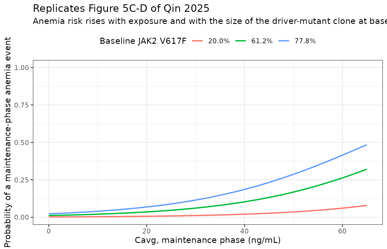
p_anemia <- function(cav, jak) {
  1 / (1 + exp(-(-6.95416 + 0.056548 * cav + 0.041351 * jak)))
}
grid_chk <- tidyr::expand_grid(CAV = c(0, 20, 40), JAK2 = c(0, 61.2, 77.8))
chk_anemia <- grid_chk |>
  dplyr::mutate(
    `Model` = eval_er(mod_anemia, CAV,
                      extra = tibble::tibble(TUM_JAK2_V617F_VAF = JAK2),
                      out = "prob_anemia"),
    `Closed form` = p_anemia(CAV, JAK2)) |>
  dplyr::rename("Cavg, maintenance (ng/mL)" = CAV,
                "Baseline JAK2 V617F (%)" = JAK2,
                "Model P(anemia)" = Model)
#> Warning: There was 1 warning in `dplyr::mutate()`.
#> ℹ In argument: `Model = eval_er(...)`.
#> Caused by warning:
#> ! multi-subject simulation without without 'omega'
knitr::kable(chk_anemia, digits = 4,
             caption = paste(
               "Maintenance-phase anemia probabilities against the closed",
               "form. Both sides evaluate the same fixed coefficients, so",
               "this is a pure numerical-error check and the tolerance is",
"machine precision."))| Cavg, maintenance (ng/mL) | Baseline JAK2 V617F (%) | Model P(anemia) | Closed form |
|---|---|---|---|
| 0 | 0.0 | 0.0010 | 0.0010 |
| 0 | 61.2 | 0.0119 | 0.0119 |
| 0 | 77.8 | 0.0233 | 0.0233 |
| 20 | 0.0 | 0.0029 | 0.0029 |
| 20 | 61.2 | 0.0358 | 0.0358 |
| 20 | 77.8 | 0.0687 | 0.0687 |
| 40 | 0.0 | 0.0091 | 0.0091 |
| 40 | 61.2 | 0.1033 | 0.1033 |
| 40 | 77.8 | 0.1862 | 0.1862 |
Two further checks pin the two things most easily lost in transcription: the scale of the allele-burden column and the sign of both slopes. Each is arithmetic on fixed published coefficients, so each is exact.
# 1. SCALE. The coefficient is per PERCENTAGE POINT, so a 10-point increase
#    multiplies the odds by exp(0.041351*10) = 1.512. Supplying the 0-1
#    FRACTION instead of the per cent would shrink every covariate
#    contribution 100-fold; at the A19-201 median that is the difference
#    between a 25-fold and a 1.03-fold odds multiplier.
odds <- function(p) p / (1 - p)
or_10pt <- odds(p_anemia(30, 70)) / odds(p_anemia(30, 60))
or_median_burden <- odds(p_anemia(30, 77.8)) / odds(p_anemia(30, 0))
or_fraction_bug <- odds(p_anemia(30, 0.778)) / odds(p_anemia(30, 0))

# 2. SIGN. Both slopes are positive: higher exposure and a larger baseline
#    clone each RAISE anemia risk. Qin 2025 Results 3.4: "anemia increased
#    with increasing exposure and baseline JAK2 V617F".
mono_cav <- diff(p_anemia(cav_grid, 61.2))
mono_jak <- diff(p_anemia(30, seq(0, 100, by = 1)))

knitr::kable(
  tibble::tibble(
    Quantity = c("Odds ratio per 10 percentage points of baseline burden",
                 "Odds ratio at the A19-201 median burden (77.8%) vs 0%",
                 "Same, if the 0-1 fraction were supplied by mistake"),
    Value = c(or_10pt, or_median_burden, or_fraction_bug)),
  digits = 3,
  caption = paste(
    "The third row is the failure mode this check exists to catch: a",
    "fraction-scaled column collapses a 25-fold effect to essentially",
"nothing, and would not otherwise be visible in the output."))| Quantity | Value |
|---|---|
| Odds ratio per 10 percentage points of baseline burden | 1.512 |
| Odds ratio at the A19-201 median burden (77.8%) vs 0% | 24.956 |
| Same, if the 0-1 fraction were supplied by mistake | 1.033 |
PKNCA validation
# IMPORTANT: filter on !is.na(Cc) only. Adding `time > 0` or `Cc > 0` would drop
# the time-zero row PKNCA needs to anchor AUC0-*.
sim_nca <- dplyr::bind_rows(
  sim_single |> dplyr::select(id, time, Cc, treatment),
  sim_multi  |> dplyr::select(id, time, Cc, treatment)) |>
  dplyr::filter(!is.na(Cc))

# Guarantee a time = 0 row per (treatment, id); pre-dose Cc = 0 is correct for
# an extravascular model with an absorption lag.
sim_nca <- dplyr::bind_rows(
  sim_nca,
  sim_nca |> dplyr::distinct(id, treatment) |>
    dplyr::mutate(time = 0, Cc = 0)) |>
  dplyr::distinct(treatment, id, time, .keep_all = TRUE) |>
  dplyr::arrange(treatment, id, time)

dose_df <- dplyr::bind_rows(
  tibble::tibble(id = coh_healthy$id, time = 0, amt = 300,
                 treatment = "300 ug single dose (healthy)"),
  tidyr::expand_grid(id = coh_pv$id, k = seq_along(dose_times)) |>
    dplyr::mutate(time = dose_times[k], amt = amt_fast[k],
                  treatment = "Fast titration (A20-202)") |>
    dplyr::select(id, time, amt, treatment),
  tidyr::expand_grid(id = coh_pv$id, k = seq_along(dose_times)) |>
    dplyr::mutate(time = dose_times[k], amt = amt_slow[k],
                  treatment = "Slow titration (A19-201)") |>
    dplyr::select(id, time, amt, treatment))

conc_obj <- PKNCA::PKNCAconc(as.data.frame(sim_nca), Cc ~ time | treatment + id,
                             concu = "ng/mL", timeu = "day")
dose_obj <- PKNCA::PKNCAdose(as.data.frame(dose_df), amt ~ time | treatment + id,
                             doseu = "ug")

intervals <- dplyr::bind_rows(
  # Single dose: Cmax and Tmax against the Figure S2 VPC panel.
  tibble::tibble(treatment = "300 ug single dose (healthy)",
                 start = 0, end = 30,
                 cmax = TRUE, tmax = TRUE, auclast = TRUE, cav = FALSE),
  # Weeks 0-24 average concentration, the exact exposure metric of the
  # week-24 exposure-response models (Qin 2025 Methods 2.4.6.1).
  tibble::tibble(treatment = c("Fast titration (A20-202)",
                               "Slow titration (A19-201)"),
                 start = 0, end = 168,
                 cmax = FALSE, tmax = FALSE, auclast = TRUE, cav = TRUE)) |>
  as.data.frame()

nca_res <- PKNCA::pk.nca(PKNCA::PKNCAdata(conc_obj, dose_obj,
                                          intervals = intervals))
nca_all <- as.data.frame(nca_res)
Structural check: interval-average concentration equals dose rate over clearance
For a linear one-compartment model the average concentration over a
long multiple-dose window is total dose / (CL * duration).
Ropeg is not linear, but the target-mediated arm is small:
kint * complex can never exceed kint * Rtot,
which is 0.0223 * 0.317 = 0.0071 ng/mL/day at baseline
against a linear elimination rate of 0.229 * Cc. The
identity should therefore hold to within a fraction of a per cent, and
the size of the residual is a direct measurement of how much work the
TMDD arm is doing.
cav_pknca <- nca_all |>
  dplyr::filter(PPTESTCD == "cav", start == 0, end == 168) |>
  dplyr::select(treatment, id, cav = PPORRES)

cl_ind <- dplyr::bind_rows(
  sim_fast |> dplyr::distinct(id, cl) |>
    dplyr::mutate(treatment = "Fast titration (A20-202)"),
  sim_slow |> dplyr::distinct(id, cl) |>
    dplyr::mutate(treatment = "Slow titration (A19-201)"))

dose_0_24 <- dose_df |>
  dplyr::filter(time < 168) |>
  dplyr::group_by(treatment, id) |>
  dplyr::summarise(total = sum(amt), .groups = "drop")

ident <- cav_pknca |>
  dplyr::inner_join(cl_ind, by = c("treatment", "id")) |>
  dplyr::inner_join(dose_0_24, by = c("treatment", "id")) |>
  dplyr::mutate(closed = total / (cl * 168),
                pct_diff = 100 * (cav - closed) / closed)

ident |>
  dplyr::group_by(treatment) |>
  dplyr::summarise(`Median % difference` = stats::median(pct_diff),
                   `50th pct |% diff|` = stats::quantile(abs(pct_diff), 0.5),
                   `75th pct |% diff|` = stats::quantile(abs(pct_diff), 0.75),
                   `90th pct |% diff|` = stats::quantile(abs(pct_diff), 0.9),
                   .groups = "drop") |>
  knitr::kable(digits = 2,
               caption = paste(
                 "PKNCA Cav against total dose / (CL * 168 days). The identity",
                 "holds at the centre but has a long right tail; the tail is a",
"measurement, not an error - see below."))| treatment | Median % difference | 50th pct |% diff| | 75th pct |% diff| | 90th pct |% diff| |
|---|---|---|---|---|
| Fast titration (A20-202) | -3.45 | 4.70 | 9.54 | 17.71 |
| Slow titration (A19-201) | -3.98 | 5.81 | 10.58 | 22.26 |
The median difference is a couple of per cent, which is the structural check: a mis-transcribed clearance, dose or unit would move the whole distribution by tens of per cent. The spread, however, is large, and it is worth understanding rather than tolerating.
Two things make the identity inexact per subject, and both are real features of the published model rather than numerical noise:
- Linear elimination acts on the free concentration,
while
Ccand hence PKNCA’sCavare the total concentration. Wherever a non-trivial fraction of drug is target-bound, total exceeds free andCav * CL * Tovershoots the dose. -
Rtot0carries 272% CV, the largest random effect in the model. A subject two SD above the median has a binding capacity of several ng/mL rather than 0.317, so the bound fraction, and with it the overshoot, is far larger.
So the width of this distribution is a direct read-out of how unevenly the target-mediated arm is distributed across the population. The assertion below is therefore on the centre only, per this repository’s rule against asserting on the extreme of a random cohort.
# Structural: both sides use the same drawn CL, so a shifted centre would mean a
# mis-transcribed clearance, dose or unit.
stopifnot(abs(stats::median(ident$pct_diff)) < 5)

# The deterministic typical-value subject removes the Rtot0 spread entirely and
# is reproducible across machines, so it takes the tight bound.
typ_ev <- dplyr::bind_rows(
  tibble::tibble(id = 1L, time = dose_times[dose_times < 168],
                 amt = amt_fast[dose_times < 168], evid = 1L, cmt = "depot"),
  tibble::tibble(id = 1L, time = seq(0, 168, by = 0.5),
                 amt = NA_real_, evid = 0L, cmt = NA_character_)) |>
  dplyr::arrange(time, dplyr::desc(evid)) |>
  dplyr::mutate(BMI = 23.1, DIS_HEALTHY = 0)
typ <- rxode2::rxSolve(rxode2::zeroRe(mod_pk), typ_ev, returnType = "data.frame")
#> ℹ omega/sigma items treated as zero: 'etalka', 'etalcl', 'etalvc', 'etalrtot0', 'etalkint'
typ_cav <- sum(diff(typ$time) *
                 (utils::head(typ$Cc, -1) + utils::tail(typ$Cc, -1)) / 2) / 168
typ_closed <- sum(amt_fast[dose_times < 168]) / (0.753 * 168)

knitr::kable(
  tibble::tibble(
    Quantity = "Typical subject, weeks 0-24",
    `Cav from the solved profile (ng/mL)` = typ_cav,
    `Total dose / (CL * T) (ng/mL)` = typ_closed,
    `% difference` = 100 * (typ_cav - typ_closed) / typ_closed),
  digits = 3,
  caption = paste(
    "At the typical value the residual is the target-mediated arm alone,",
"and it is small - consistent with the elimination-flux split below."))| Quantity | Cav from the solved profile (ng/mL) | Total dose / (CL * T) (ng/mL) | % difference |
|---|---|---|---|
| Typical subject, weeks 0-24 | 44.894 | 44.267 | 1.416 |
Structural check: the drug-free system relaxes from X0 to Xss
With no dose, each pharmacodynamic model must relax monotonically from its initial value to its steady-state value. This is exact and deterministic, so it is asserted tightly.
baseline_ev <- tibble::tibble(id = 1L, time = seq(0, 2000, by = 5),
                              evid = 0L, amt = NA_real_,
                              BMI = 23.1, DIS_HEALTHY = 0)
zr <- function(m) rxode2::rxSolve(rxode2::zeroRe(m), baseline_ev,
                                  returnType = "data.frame")
b_hct <- zr(mod_hct); b_plt <- zr(mod_plt); b_wbc <- zr(mod_wbc)
#> ℹ omega/sigma items treated as zero: 'etalka', 'etalcl', 'etalvc', 'etalrtot0', 'etalkint', 'etalrbase_ss', 'etalic50', 'etalktr', 'etalrbase'
#> ℹ omega/sigma items treated as zero: 'etalka', 'etalcl', 'etalvc', 'etalrtot0', 'etalkint', 'etalrbase_ss', 'etalic50', 'etalkout', 'etalrbase'
#> ℹ omega/sigma items treated as zero: 'etalka', 'etalcl', 'etalvc', 'etalrtot0', 'etalkint', 'etalrbase_ss', 'etalic50', 'etalkout', 'etalrbase'

base_chk <- tibble::tibble(
  Endpoint = c("HCT", "PLT", "WBC"),
  `Start (model)` = c(b_hct$hct[1], b_plt$circ_plt[1], b_wbc$circ_wbc[1]),
  `Published X0` = c(0.459, 477, 11.4),
  `End (model)` = c(dplyr::last(b_hct$hct), dplyr::last(b_plt$circ_plt),
                    dplyr::last(b_wbc$circ_wbc)),
  `Published Xss` = c(0.489, 332, 6.72))
knitr::kable(base_chk, digits = 3,
             caption = paste(
               "Drug-free relaxation. Hematocrit rises toward its steady state",
"because HCTss > HCT0; platelets and white cells fall."))| Endpoint | Start (model) | Published X0 | End (model) | Published Xss |
|---|---|---|---|---|
| HCT | 0.459 | 0.459 | 0.489 | 0.489 |
| PLT | 477.000 | 477.000 | 332.000 | 332.000 |
| WBC | 11.400 | 11.400 | 6.720 | 6.720 |
Comparison against published NCA
Qin 2025 publishes no non-compartmental analysis table. The reference values below are therefore read off the paper’s own figures and are labelled as such; they are used to check the packaged model against the paper’s graphical output, not as published point estimates.
nca_value <- function(trt, code, start_, end_) {
  v <- nca_all |>
    dplyr::filter(treatment == trt, PPTESTCD == code,
                  start == start_, end == end_) |>
    dplyr::pull(PPORRES)
  if (length(v) == 0L || all(is.na(v))) {
    stop("no values for ", trt, " / ", code)
  }
  stats::median(v, na.rm = TRUE)
}

single_arm <- "300 ug single dose (healthy)"
simulated_nca <- tibble::tribble(
  ~treatment,                 ~PPTESTCD, ~PPORRES,
  single_arm,                 "cmax",    nca_value(single_arm, "cmax", 0, 30),
  single_arm,                 "tmax",    nca_value(single_arm, "tmax", 0, 30),
  "Fast titration (A20-202)", "cav",     nca_value("Fast titration (A20-202)", "cav", 0, 168)
)
stopifnot(nrow(simulated_nca) == 3L, !anyNA(simulated_nca$PPORRES))
published <- tibble::tribble(
  ~treatment,                 ~PPTESTCD, ~PPORRES,
  # Figure S2, panel DOSEUG == 300: the observed median profile peaks at
  # 25-30 ng/mL, midpoint 27.5, at 100-150 h after dose, midpoint 125 h
  # (5.21 days in the model's day time unit).
  single_arm,                 "cmax",    27.5,
  single_arm,                 "tmax",    125 / 24,
  # Figure 3A/3B, grey boxplot strip: the A20-202 median Cavg,0-24W is about
  # 37.5 ng/mL.
  "Fast titration (A20-202)", "cav",     37.5
)

cmp <- nlmixr2lib::ncaComparisonTable(
  simulated = simulated_nca,
  reference = published,
  by        = "treatment",
  units     = c(cmax = "ng/mL", tmax = "day", cav = "ng/mL"),
  tolerance_pct = 20)

knitr::kable(
  cmp,
  caption = paste(
    "Simulated versus figure-derived reference values. The single-dose rows",
    "compare against the Figure S2 visual predictive check; the fast-titration",
    "row compares the weeks 0-24 average concentration against the Figure 3",
    "exposure strip. * differs from the reference by more than 20%."),
align = c("l", "l", "r", "r", "r"))| NCA parameter | treatment | Reference | Simulated | % diff |
|---|---|---|---|---|
| Cmax (ng/mL) | 300 ug single dose (healthy) | 27.5 | 27.7 | +0.6% |
| Tmax (day) | 300 ug single dose (healthy) | 5.21 | 5.5 | +5.6% |
| Cavg (ng/mL) | Fast titration (A20-202) | 37.5 | 46 | +22.6%* |
attr(cmp, "footnote")
#> [1] "* differs from reference by more than ±20%."
The fast-titration arm is the fair comparison for Cav,
because A20-202’s titration is fully specified by protocol (250, 350,
then 500 ug) and does not depend on individual response. The simulated
value runs above the observed median, which is expected: the simulation
applies the protocol schedule to every subject, whereas real patients
had dose reductions for tolerability.
cav_by_arm <- cav_pknca |>
  dplyr::group_by(treatment) |>
  dplyr::summarise(`Median Cav 0-24 wk (ng/mL)` = stats::median(cav),
                   `Q1` = stats::quantile(cav, 0.25),
                   `Q3` = stats::quantile(cav, 0.75), .groups = "drop") |>
  dplyr::mutate(`Figure 3 observed median` = c(37.5, 20))
knitr::kable(cav_by_arm, digits = 1,
             caption = paste(
               "Weeks 0-24 average concentration by arm. The slow-titration",
               "arm is simulated on the PROTOCOL schedule (100 ug, +50 ug",
               "q2w to 500 ug), which climbs faster than the A19-201 patients",
               "actually did: Qin 2025 titrated 'until a response was",
"achieved', so many patients stopped well below 500 ug."))| treatment | Median Cav 0-24 wk (ng/mL) | Q1 | Q3 | Figure 3 observed median |
|---|---|---|---|---|
| Fast titration (A20-202) | 46.0 | 36.3 | 56.9 | 37.5 |
| Slow titration (A19-201) | 34.3 | 27.7 | 41.9 | 20.0 |
# Direction only for the slow arm: the protocol schedule is an upper bound on
# what A19-201 patients actually received, so the simulated value must exceed
# the observed median rather than match it.
slow_med <- cav_by_arm$`Median Cav 0-24 wk (ng/mL)`[
  cav_by_arm$treatment == "Slow titration (A19-201)"]
fast_med <- cav_by_arm$`Median Cav 0-24 wk (ng/mL)`[
  cav_by_arm$treatment == "Fast titration (A20-202)"]
stopifnot(slow_med > 20, slow_med < fast_med)
How much work is the target-mediated arm doing?
The estimated binding capacity is small
(Rtot0 = 0.317 ng/mL) relative to the concentrations the
drug reaches, so the target-mediated pathway is a
low-concentration phenomenon: it shapes the tail, not
the peak. This is worth stating plainly, because “TMDD model” can
suggest a dominant nonlinearity that these estimates do not support.
share <- sim_single |>
  # Drop the pre-lag rows, where both fluxes are exactly zero and the share is
  # 0/0 rather than small.
  dplyr::filter(time > exp(mod_pk$theta[["ltlag"]])) |>
  dplyr::group_by(time) |>
  dplyr::summarise(
    linear = stats::median(cl * cfree),
    tmdd   = stats::median(kint * complex * vc), .groups = "drop") |>
  dplyr::mutate(pct_tmdd = 100 * tmdd / (linear + tmdd))

ggplot(share, aes(24 * time, pct_tmdd)) +
  geom_line(linewidth = 0.8) +
  labs(x = "Time after a single 300 ug dose (h)",
       y = "Target-mediated share of total elimination (%)",
       title = "The target-mediated arm matters only in the tail") +
  theme_bw()
knitr::kable(
  share |>
    dplyr::filter(time %in% c(5, 10, 20, 30)) |>
    dplyr::rename(`Time (days)` = time,
                  `Linear (ng/mL/day)` = linear,
                  `Target-mediated (ng/mL/day)` = tmdd,
                  `TMDD share (%)` = pct_tmdd),
  digits = 4,
caption = "Elimination-flux split after a single 300 ug dose (medians).")| Time (days) | Linear (ng/mL/day) | Target-mediated (ng/mL/day) | TMDD share (%) |
|---|---|---|---|
| 5 | 19.2343 | 0.0438 | 0.2271 |
| 10 | 12.4153 | 0.0708 | 0.5672 |
| 20 | 4.0693 | 0.1159 | 2.7700 |
| 30 | 0.7618 | 0.1230 | 13.9008 |
stopifnot(share$pct_tmdd[share$time == 5] < 5)A related consequence worth flagging for anyone reading the state
trajectories: because kint (0.0223/day) is far smaller than
kdeg (0.51/day), the drug-target complex is long-lived and
the total target state rises under treatment even while
the binding capacity parameter Rtot declines from
Rtot0 to Rtot,SS. Both behaviours are
consequences of the published equations; they are not in conflict,
because Qin 2025’s Rtot is the capacity that sets
ksyn, not the modelled total-target state.
Assumptions and deviations
- Time unit. The published tables label the rate constants per hour; they are per day. See Errata for four pieces of evidence. Nothing was rescaled; only the unit label was corrected.
- Absorption lag and TSTART are carried in days for internal consistency with the rest of Table 2. Both readings are numerically immaterial (see Errata).
- PLT and WBC parameters are taken from Table 3, not from the conflicting Discussion restatement. See Errata for the reasoning.
-
Transit-compartment initial condition. Qin 2025
reports
HCT0as the initial hematocrit but does not print the initial condition of the transit compartment in Figure 1B. Both states are started atHCT0, which is the reading under which an untreated patient relaxes monotonically fromHCT0toHCTssand which reproduces the small early rise then fall of the Figure 2A median profile. Starting the transit compartment atHCTssinstead would produce a markedly larger early rise than Figure 2A shows. -
kinis derived, not published. Methods 2.4.1 states that the zero-order production constants “were calculated”; they are reconstructed here askin = ktr * HCTssandkin = kout * Xss, the values that make the published steady state the drug-free steady state. -
Sequential fit encoding. In the three PK-PD models
every PK parameter, including the inter-individual variances, is wrapped
in
fixed(), and the PK residual-error terms are omitted, because the sequential objective function covers only the pharmacodynamic observations. - Covariance versus correlation. Table 3’s “Covariance of …” rows are read as covariances. All three are admissible as covariances; as correlations they would also be admissible, so the printed label is the only discriminator.
-
Residual error for the exposure-response models is not
published. The logistic models use an exact Bernoulli
likelihood and the two JAK2 regressions report no residual SD, RSS or
R^2. Each of the six exposure-response models therefore carries a small
fixed(0.001)additive residual that exists only so that rxode2 has an error model to attach to the typical-value prediction. It is not a published quantity and must not be used to characterise prediction uncertainty. -
Slow-titration regimen. A19-201’s schedule is
titrate-to-response, so the per-patient dose history cannot be
reconstructed from the publication. The slow arm is simulated on the
protocol-specified schedule, which is an upper bound; this is why its
simulated
Cavexceeds the Figure 3 observed median and why only the fast arm is used in the NCA comparison. -
Reference values are figure-derived. Qin 2025
publishes no NCA table. The
cmax,tmaxandcavreference values are read off Figures S2 and 3 and are labelled as digitised throughout. - Cohort covariate distributions are log-normal draws truncated to the Table 1 study-level ranges; Qin 2025 does not publish the joint covariate distribution, and only BMI affects the model.
-
DIS_HEALTHYin the PK-PD models must be 0 for every subject: only PV patients contributed hematologic observations. The column is retained so the inherited PK layer matches the standalone PK model exactly. -
New register entries. This extraction registers the
PD-output canonicals
hct,prob_chr,prob_alt_increase,prob_ast_increaseanddjak2v617fininst/references/compartment-names.md, and the covariate canonicalTUM_JAK2_V617F_VAFininst/references/covariate-columns.md. The platelet and white-cell states reuse the existingcirc_pltandcirc_wbccanonicals rather than minting synonyms, and the anemia model’s exposure column reusesCAV. -
Seven mutually non-interchangeable
CAVcolumns. All seven E-R models name their exposure metricCAV, but the averaging windows differ and the values are not substitutable: weeks 0-24 and weeks 0-52 from first dose for the efficacy models, a study-dependent titration-phase window (weeks 0-16 in A19-201, weeks 0-6 in A20-202) for the transaminase models, and that window’s complement – the maintenance phase to end of treatment – for the anemia model. A data assembler must build each column separately, per study.
The eleventh model and its new covariate canonical
Qin 2025’s eleventh model, the maintenance-phase
anemia exposure-safety logistic regression (Results 3.4), was
deferred on first extraction and is now packaged as
Qin_2025_ropeginterferon_anemia. The delay was a naming
decision, not a reporting gap: the model is fully reported, but its
covariate – baseline JAK2 V617F allele burden, in per
cent – had no canonical entry in
inst/references/covariate-columns.md, and minting one
requires a maintainer decision.
It is registered here as
TUM_JAK2_V617F_VAF (maintainer-ratified),
a continuous somatic variant allele frequency on a 0-100 per cent scale.
The three near neighbours it is deliberately not filed
under:
-
SNP_JAK2_RS77375493. JAK2 V617F does have an rsid, so this would be mechanically well formed under the acceptedSNP_<GENE>_RS<rsid>naming family. But every registeredSNP_*column carries a germline genotype – an allele count or a carrier indicator – whereas this is a somatic clone fraction that moves under treatment. A value of61.2under aSNP_name would be ambiguous between an allele count and a per cent. -
TUM_<GENE>_MUT(TUM_EGFR_MUT,TUM_TP53_MUT,TUM_IGHV_MUT, …). The right family, but every existing member is a binary 0/1 presence call. This is their continuous sibling, and founds aTUM_<GENE>_<VARIANT>_VAFsub-family. The variant token is kept because JAK2 exon 12 mutations are a separate assayable abnormality in polycythaemia vera, which Qin 2025’s Discussion names explicitly. -
CTDNA. Circulating tumour DNA burden in mutant molecules per mL of plasma – a different analyte, assay and unit. Worth flagging because a fuzzy canonical lookup of “baseline JAK2 V617F allele burden” returnsCTDNAas a confident but wrong match.
The prob_anemia output canonical the model needs already
existed.
The per-cent scale is load-bearing. The coefficient
0.041351 is per percentage point, so a column supplied as a 0-1 fraction
understates every covariate contribution 100-fold – silently, since the
result is still a probability in range. At the A19-201 median burden
that is the difference between a 25-fold and a 1.03-fold odds
multiplier. The anemia-scale-check chunk above asserts on
exactly this. Qin 2025 Table 1’s JAK2 V617F (%) row also
carries a trap of its own: the Overall column reads 31.9% because it
pools in the 48 phase I healthy volunteers, who are 0 by construction,
so the patient-population summary is the per-study medians (77.8% and
61.2%) and not the Overall figure.