Pentobarbital (Ketharanathan 2023)

Model and source

• Citation: Ketharanathan N, Lili A, Penning de Vries JM, Wildschut ED, de Hoog M, Koch BCP, de Winter BCM. A Population Pharmacokinetic Model of Pentobarbital for Children with Status Epilepticus and Severe Traumatic Brain Injury. Clin Pharmacokinet. 2023;62(7):1011-1022. doi:10.1007/s40262-023-01249-z.
• Description: One-compartment population PK model for intravenous pentobarbital in critically ill children admitted to a paediatric intensive care unit for refractory status epilepticus or severe traumatic brain injury. Body weight is allometrically scaled onto clearance (exponent 0.75) and central volume (exponent 1) against a 70 kg reference, with both exponents fixed. Serum creatinine enters clearance as a power function normalised to 36 umol/L, and C-reactive protein as a second power function normalised to 70 mg/L that is switched on only at or above that threshold. Together the two covariates removed 84% of the inter-individual variability in clearance present in the base model.
• Article: https://doi.org/10.1007/s40262-023-01249-z
• Supplement (NONMEM control stream of the final model, Supplementary Fig. 3): https://doi.org/10.1007/s40262-023-01249-z (Electronic Supplementary Material)

Ketharanathan and colleagues report the first population PK analysis of intravenous pentobarbital in critically ill children. Pentobarbital is used in the paediatric intensive care unit for two quite different indications – refractory status epilepticus (SE), where the therapeutic endpoint is burst suppression on EEG, and severe traumatic brain injury (sTBI), where the endpoint is intracranial-pressure control. The drug has a narrow therapeutic window and a literature half-life spanning 5-50 h, so the practical question the paper asks is how to keep concentrations inside a 20-40 mg/L safety margin.

The headline finding is that two routinely-measured markers – serum creatinine and C-reactive protein (CRP) – between them explain 84% of the inter-individual variability in clearance, and that patients with elevated values do not reach steady state but instead climb into the toxic range on standard weight-based dosing.

Population

The model was fitted to 178 pentobarbital serum concentrations from 36 children treated at a single 28-bed paediatric intensive care unit (Erasmus MC-Sophia Children’s Hospital, Rotterdam) between January 2007 and September 2021. Twenty-two children were treated for refractory status epilepticus and 14 for severe traumatic brain injury defined by a Glasgow Coma Scale of 8 or less with refractory intracranial hypertension.

The two diagnostic groups differ sharply in age and size (Table 1 of the source). The SE group had a median age of 0.31 years (IQR 0.05-3.73) and a median weight of 6.3 kg (IQR 3-19); the sTBI group had a median age of 12 years (IQR 0.3-16) and a median weight of 40 kg (IQR 5-87). Pooled across both, the median age was 1.3 years and the median weight 10 kg. Median serum creatinine was 23 umol/L in the SE group and 49 umol/L in the sTBI group; median CRP was 32.5 mg/L and 131.5 mg/L respectively. Diagnosis itself was tested as a covariate and was not retained, so the packaged model applies to both indications.

A separate cohort of 9 children (6 sTBI, 3 SE; 60 samples, October 2019 - February 2023) was used for external validation by stratified VPC and is not part of the 36 subjects fitted here. Patients receiving ECMO or concurrent haemodialysis were excluded.

The same information is available programmatically via the model’s population metadata (readModelDb("Ketharanathan_2023_pentobarbital")()$population).

Source trace

The per-parameter origin is recorded as an in-file comment next to each ini() entry in inst/modeldb/specificDrugs/Ketharanathan_2023_pentobarbital.R. The table below collects them in one place for review. “Supplementary Fig. 3” is the NONMEM control stream of the final model in the Electronic Supplementary Material.

Equation / parameter	Value	Source location
lcl (CL at 70 kg)	3.59 L/h	Table 2, “Final model” column (11% RSE; bootstrap 2.80-4.74). $THETA 1 in Supplementary Fig. 3
lvc (Vc at 70 kg)	142 L	Table 2, “Final model” column (6% RSE; bootstrap 120-158). $THETA 2 in Supplementary Fig. 3
e_wt_cl	0.75 (fixed)	Sect. 2.4.1 “fixed exponents (0.75 for CL and 1 for Vd)”; hardcoded in TVCL=THETA(1)*(WGHT/70)**0.75
e_wt_vc	1 (fixed)	Sect. 2.4.1; hardcoded in V=THETA(2)*(WGHT/70)
e_creat_cl	-0.919	Table 2 “Creatinine effect on CL” (21% RSE; bootstrap -1.192 to -0.242). $THETA 3
e_crp_cl	-0.883	Table 2 “C-reactive protein effect on CL”, footnote “*If CRP>70 mg/L” (14% RSE; bootstrap -1.25 to -0.613). $THETA 4
etalcl (IIV on CL)	0.121 (var)	$OMEGA in Supplementary Fig. 3; Table 2 reports sqrt(0.121) = 34.8% (24% RSE, 23% shrinkage)
addSd	7.22 mg/L	Table 2 “Additional (mg/L)” (10% RSE, 6% shrinkage; bootstrap 5.72-8.54). $THETA 5
Creatinine normalisation	36 umol/L	Printed CL equation in Sect. 3.3; COV=(CREAT/36)**THETA(3)
CRP normalisation + threshold	70 mg/L	Printed CL equation in Sect. 3.3; IF(CRP.GE.70) COVCL=COV*(CRP/70)**THETA(4)
Weight reference	70 kg	Printed CL equation in Sect. 3.3; Table 2 units “L/h/70 kg”
d/dt(central) (one compartment, IV)	n/a	Sect. 3.2 “a one-compartment model was chosen”; $SUBROUTINES ADVAN1 TRANS2 with S1=V
Residual error form (additive)	n/a	Sect. 3.2 “The residual error was described as an additive error, as the proportional error was estimated close to zero” (see Assumptions below)

The full clearance equation as printed in Sect. 3.3 is

CL (L/h) = 3.59 * (Weight/70)^0.75 * (Creatinine/36)^-0.919            if CRP <= 70 mg/L
CL (L/h) = 3.59 * (Weight/70)^0.75 * (Creatinine/36)^-0.919
                                   * (CRP/70)^-0.883                    if CRP  > 70 mg/L

with weight in kg, creatinine in umol/L and CRP in mg/L.

Virtual cohort

Original observed data are not publicly available. The simulations below rebuild the exact scenarios the paper simulated, so the covariate values are taken directly from the source figure legends rather than sampled: Figs. 2, 3 and 4 all fix creatinine at 26 umol/L and CRP at or below 70 mg/L, and vary one of weight, creatinine or CRP at a time.

Note that 26 umol/L (the simulation scenario value) is not the same as 36 umol/L (the model’s creatinine normalisation constant); both appear in the paper and it is easy to conflate them.

# Build one arm as a self-contained event table.
#
# Loading doses are IV boluses (rate = 0); the maintenance infusion is a single
# dose record whose duration is amt/rate, sized to cover the whole window.
# Observation rows use cmt = "central" -- the ODE state -- so rxode2 returns the
# algebraic observable Cc as a column without renumbering compartment slots.
make_arm <- function(id, arm, wt, creat, crp,
                     rate_mgkgh, infusion_h,
                     obs_times,
                     load_mgkg = 0, n_load = 0L, load_int_h = 5 / 60) {
  dose_rows <- tibble(time = numeric(0), amt = numeric(0), rate = numeric(0))

  if (n_load > 0L) {
    dose_rows <- bind_rows(dose_rows, tibble(
      time = (seq_len(n_load) - 1L) * load_int_h,
      amt  = load_mgkg * wt,
      rate = 0
    ))
  }
  if (rate_mgkgh > 0 && infusion_h > 0) {
    dose_rows <- bind_rows(dose_rows, tibble(
      time = 0,
      amt  = rate_mgkgh * wt * infusion_h,
      rate = rate_mgkgh * wt
    ))
  }

  bind_rows(
    dose_rows |> mutate(evid = 1L),
    tibble(time = obs_times, amt = NA_real_, rate = 0, evid = 0L)
  ) |>
    mutate(id = id, cmt = "central",
           WT = wt, CREAT = creat, CRP = crp, arm = arm) |>
    arrange(time, desc(evid))
}

obs_100h <- seq(0, 100, by = 0.5)

Simulation

readModelDb() is called separately for the typical-value model because rxode2::zeroRe() modifies the object it is given; taking a fresh copy keeps the stochastic model untouched.

mod         <- readModelDb("Ketharanathan_2023_pentobarbital")
mod_typical <- rxode2::zeroRe(readModelDb("Ketharanathan_2023_pentobarbital"))
#> ℹ parameter labels from comments will be replaced by 'label()'

Replicate published figures

Figure 2 – weight-based infusion rates

Figure 2 of the source shows the continuous-infusion rate needed in each weight band to reach the 25 mg/L target, simulated at creatinine 26 umol/L and CRP at or below 70 mg/L with no loading dose. Because clearance scales with weight to the power 0.75 while the dose scales with weight to the power 1, the required weight-normalised rate falls as the child gets bigger – the point the paper makes about needing lower mg/kg/h dosing in heavier patients.

# Replicates Figure 2 of Ketharanathan 2023: weight-band infusion rates,
# creatinine 26 umol/L, CRP <= 70 mg/L, no loading dose.
fig2_spec <- tribble(
  ~wt, ~rate_mgkgh,
    5,        3.50,
   10,        3.00,
   20,        2.50,
   40,        2.00,
   60,        1.75,
   80,        1.75
)

ev_fig2 <- bind_rows(lapply(seq_len(nrow(fig2_spec)), function(i) {
  make_arm(
    id   = i,
    arm  = sprintf("%g kg - %g mg/kg/h", fig2_spec$wt[i], fig2_spec$rate_mgkgh[i]),
    wt   = fig2_spec$wt[i], creat = 26, crp = 70,
    rate_mgkgh = fig2_spec$rate_mgkgh[i], infusion_h = max(obs_100h),
    obs_times  = obs_100h
  )
}))

sim_fig2 <- rxode2::rxSolve(mod_typical, ev_fig2, keep = c("arm", "WT")) |>
  as.data.frame()
#> ℹ omega/sigma items treated as zero: 'etalcl'
#> Warning: multi-subject simulation without without 'omega'

sim_fig2 |>
  filter(!is.na(Cc)) |>
  mutate(arm = factor(arm, levels = unique(ev_fig2$arm))) |>
  ggplot(aes(time, Cc, colour = arm)) +
  geom_line(linewidth = 0.7) +
  geom_hline(yintercept = 25, linetype = "dotted") +
  scale_y_continuous(limits = c(0, 30)) +
  labs(x = "Time (h)", y = "Pentobarbital concentration (mg/L)",
       colour = NULL,
       title = "Figure 2 - pentobarbital dose adjusted for bodyweight",
       caption = "Replicates Figure 2 of Ketharanathan 2023 (target 25 mg/L, dotted line).")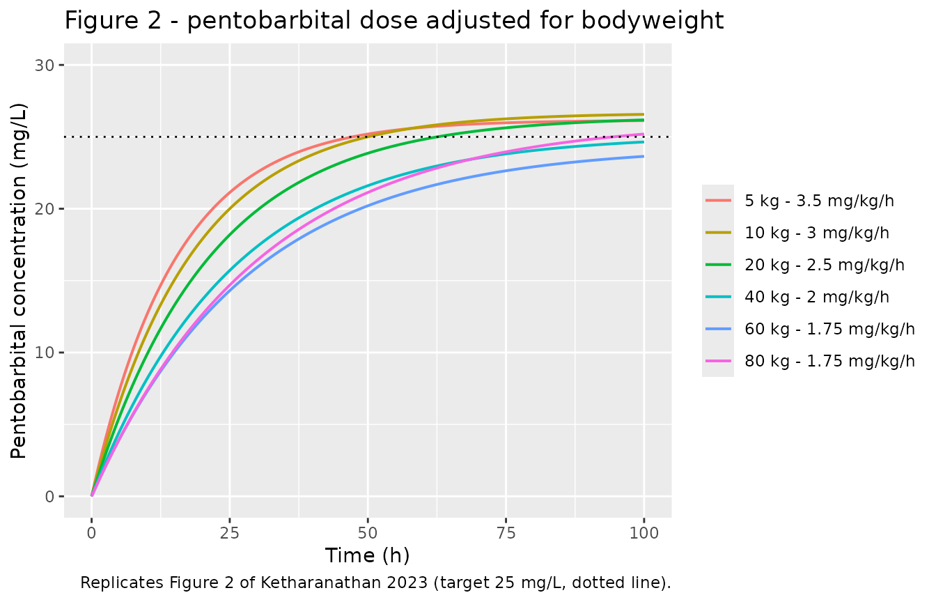

The published panel plateaus between roughly 23 and 26.5 mg/L across the six bands, with the 60 and 80 kg curves still climbing at 100 h because half-life grows with weight. The table below compares the simulated 100 h concentration against that target band.

sim_fig2 |>
  filter(!is.na(Cc), time == 100) |>
  transmute(arm, WT, `Cc at 100 h (mg/L)` = round(Cc, 1)) |>
  arrange(WT) |>
  select(-WT) |>
  rename("Weight band - infusion rate" = arm) |>
  knitr::kable(
    caption = paste("Simulated concentration at 100 h for the Figure 2 dosing",
                    "bands. Ketharanathan 2023 Figure 2 shows all six curves",
                    "between about 23 and 26.5 mg/L at 100 h.")
  )

Simulated concentration at 100 h for the Figure 2 dosing bands. Ketharanathan 2023 Figure 2 shows all six curves between about 23 and 26.5 mg/L at 100 h.

Weight band - infusion rate	Cc at 100 h (mg/L)
5 kg - 3.5 mg/kg/h	26.1
10 kg - 3 mg/kg/h	26.6
20 kg - 2.5 mg/kg/h	26.2
40 kg - 2 mg/kg/h	24.6
60 kg - 1.75 mg/kg/h	23.6
80 kg - 1.75 mg/kg/h	25.2

Figure 3 – loading-dose strategies

Figure 3 compares a single 5 mg/kg loading dose against six 5 mg/kg loading doses given 5 min apart, in each case on top of the indication-specific maintenance infusion: 3.5 mg/kg/h for a 6 kg SE patient and 2 mg/kg/h for a 40 kg sTBI patient (the median weights of the two diagnostic groups). Both scenarios use creatinine 26 umol/L and CRP at or below 70 mg/L.

Because both the loading dose and the central volume scale linearly with weight, the initial concentration after a loading dose is weight-independent in this model: 5 mg/kg into 142 * WT/70 L gives 5 * 70 / 142 = 2.46 mg/L per 5 mg/kg dose, regardless of body size.

# Replicates Figure 3 of Ketharanathan 2023: loading-dose strategies by diagnosis.
fig3_spec <- tribble(
  ~arm,                                          ~wt, ~rate_mgkgh, ~n_load,
  "sTBI 40 kg, 1 x 5 mg/kg + 2 mg/kg/h",          40,        2.00,      1L,
  "sTBI 40 kg, 6 x 5 mg/kg + 2 mg/kg/h",          40,        2.00,      6L,
  "SE 6 kg, 1 x 5 mg/kg + 3.5 mg/kg/h",            6,        3.50,      1L,
  "SE 6 kg, 6 x 5 mg/kg + 3.5 mg/kg/h",            6,        3.50,      6L
)

ev_fig3 <- bind_rows(lapply(seq_len(nrow(fig3_spec)), function(i) {
  make_arm(
    id   = i,
    arm  = fig3_spec$arm[i],
    wt   = fig3_spec$wt[i], creat = 26, crp = 70,
    rate_mgkgh = fig3_spec$rate_mgkgh[i], infusion_h = max(obs_100h),
    obs_times  = obs_100h,
    load_mgkg  = 5, n_load = fig3_spec$n_load[i]
  )
}))

sim_fig3 <- rxode2::rxSolve(mod_typical, ev_fig3, keep = "arm") |>
  as.data.frame()
#> ℹ omega/sigma items treated as zero: 'etalcl'
#> Warning: multi-subject simulation without without 'omega'

sim_fig3 |>
  filter(!is.na(Cc)) |>
  mutate(arm = factor(arm, levels = fig3_spec$arm)) |>
  ggplot(aes(time, Cc, colour = arm, linetype = arm)) +
  geom_line(linewidth = 0.7) +
  geom_hline(yintercept = 25, linetype = "dotted") +
  scale_y_continuous(limits = c(0, 30)) +
  labs(x = "Time (h)", y = "Pentobarbital concentration (mg/L)",
       colour = NULL, linetype = NULL,
       title = "Figure 3 - effect of loading dose on achieving steady state",
       caption = "Replicates Figure 3 of Ketharanathan 2023.") +
  theme(legend.position = "bottom", legend.direction = "vertical")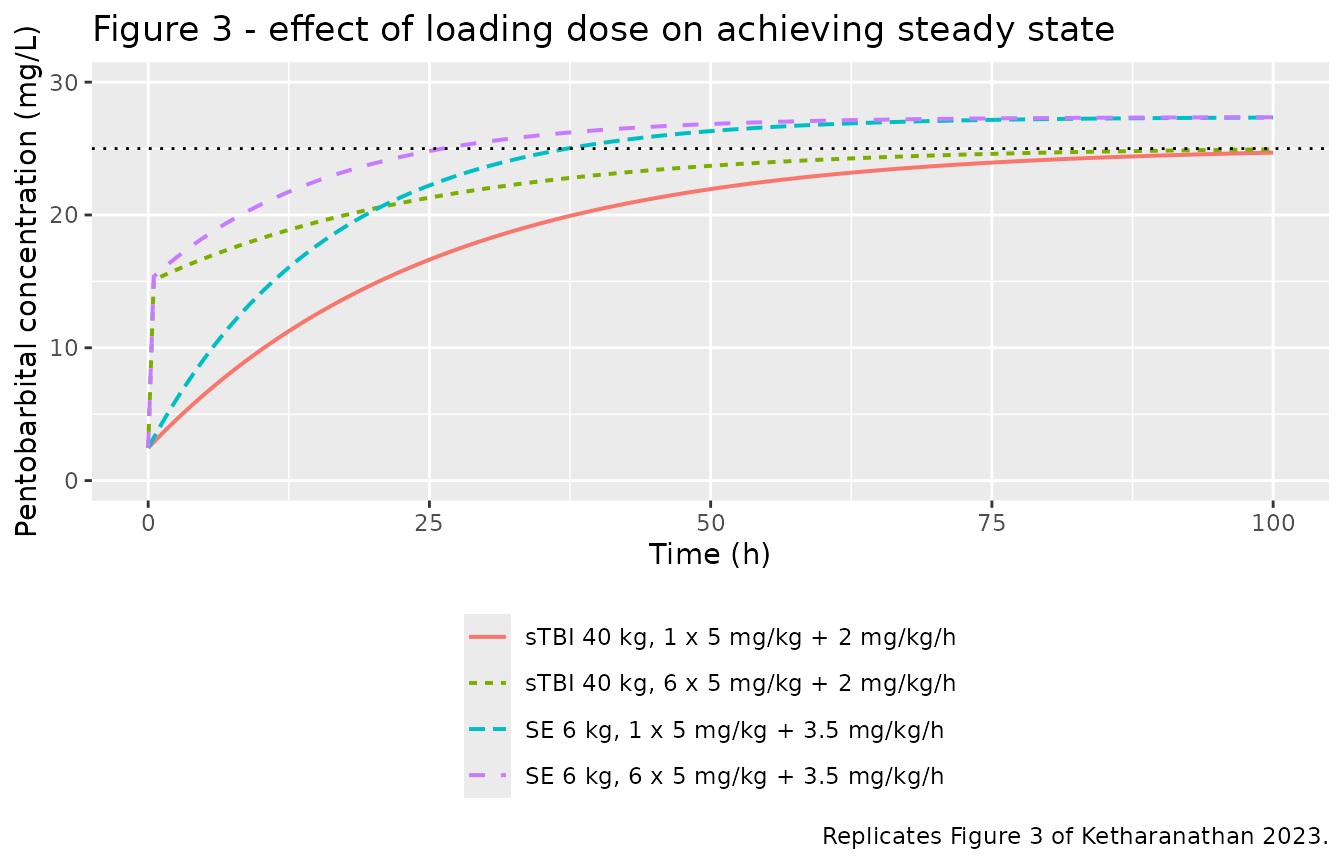

As in the published figure, the six-dose regimen lifts the concentration close to the target within the first half hour while the single loading dose contributes little, and the two SE curves plateau near 27 mg/L against 25 mg/L for the sTBI curves – the paper notes that rounding infusion rates to 0.5 mg/kg/h steps for bedside practicality overshoots the 25 mg/L target to about 27 mg/L.

Figure 4 – effect of weight, creatinine and CRP

Figure 4 fixes the infusion at 3 mg/kg/h with no loading dose and varies one covariate at a time around a 20 kg reference patient with creatinine 26 umol/L and CRP at or below 70 mg/L. It is the figure that carries the paper’s main clinical message: the covariate effects dominate the weight effect, and elevated creatinine or CRP drives concentrations well past the 40 mg/L toxicity threshold instead of reaching a plateau.

# Replicates Figure 4 of Ketharanathan 2023: one covariate varied at a time,
# 3 mg/kg/h continuous infusion, no loading dose.
fig4_spec <- bind_rows(
  tibble(panel = "A: effect of bodyweight",
         wt = c(5, 10, 20, 40, 60, 80), creat = 26, crp = 70,
         lvl = paste0(c(5, 10, 20, 40, 60, 80), " kg")),
  tibble(panel = "B: effect of creatinine",
         wt = 20, creat = c(15, 30, 60, 120, 180), crp = 70,
         lvl = paste0(c(15, 30, 60, 120, 180), " umol/L")),
  tibble(panel = "C: effect of CRP",
         wt = 20, creat = 26, crp = c(70, 100, 200, 300, 400),
         lvl = c("<=70 mg/L", paste0(c(100, 200, 300, 400), " mg/L")))
) |>
  mutate(id = row_number())

ev_fig4 <- bind_rows(lapply(seq_len(nrow(fig4_spec)), function(i) {
  make_arm(
    id   = fig4_spec$id[i],
    arm  = paste(fig4_spec$panel[i], fig4_spec$lvl[i], sep = " | "),
    wt   = fig4_spec$wt[i], creat = fig4_spec$creat[i], crp = fig4_spec$crp[i],
    rate_mgkgh = 3, infusion_h = max(obs_100h),
    obs_times  = obs_100h
  )
}))

sim_fig4 <- rxode2::rxSolve(mod_typical, ev_fig4, keep = "arm") |>
  as.data.frame() |>
  filter(!is.na(Cc)) |>
  separate_wider_delim(arm, delim = " | ", names = c("panel", "lvl"))
#> ℹ omega/sigma items treated as zero: 'etalcl'
#> Warning: multi-subject simulation without without 'omega'

sim_fig4 |>
  mutate(lvl = factor(lvl, levels = unique(fig4_spec$lvl))) |>
  ggplot(aes(time, Cc, colour = lvl)) +
  geom_line(linewidth = 0.7) +
  geom_hline(yintercept = 40, linetype = "dotted") +
  facet_wrap(~panel) +
  coord_cartesian(ylim = c(0, 100)) +
  labs(x = "Time (h)", y = "Pentobarbital concentration (mg/L)", colour = NULL,
       title = "Figure 4 - effect of bodyweight, creatinine and CRP",
       caption = paste("Replicates Figure 4 of Ketharanathan 2023",
                       "(3 mg/kg/h infusion; dotted line = 40 mg/L toxicity threshold).")) +
  theme(legend.position = "bottom")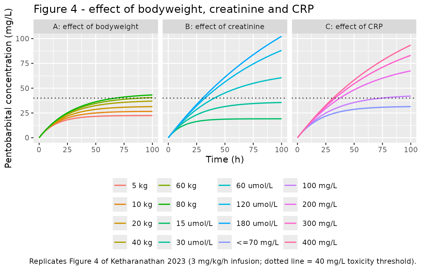

Table 4 – CRP-based dose adjustment

Table 4 of the source tabulates the recommended maintenance-infusion dose as a percentage of the original dose for CRP values above 70 mg/L. Because the maintenance dose required to hold a given steady-state concentration is proportional to clearance, that percentage is exactly the CRP clearance multiplier (CRP/70)^e_crp_cl. Reproducing the table therefore checks the packaged e_crp_cl value directly against a published number, with no simulation in between.

e_crp_cl <- rxode2::rxode(readModelDb("Ketharanathan_2023_pentobarbital"))$theta[["e_crp_cl"]]
#> ℹ parameter labels from comments will be replaced by 'label()'

tibble(
  crp       = c(100, 200, 300, 400),
  published = c(73, 40, 28, 21)
) |>
  mutate(model = round(100 * (crp / 70)^e_crp_cl)) |>
  rename(
    "C-reactive protein (mg/L)"        = crp,
    "Published dose adjustment (%)"    = published,
    "Model-derived dose adjustment (%)" = model
  ) |>
  knitr::kable(
    caption = paste("Reproduction of Table 4 of Ketharanathan 2023: pentobarbital",
                    "continuous-infusion dose as a percentage of the original dose",
                    "at CRP > 70 mg/L.")
  )

Reproduction of Table 4 of Ketharanathan 2023: pentobarbital continuous-infusion dose as a percentage of the original dose at CRP > 70 mg/L.

C-reactive protein (mg/L)	Published dose adjustment (%)	Model-derived dose adjustment (%)
100	73	73
200	40	40
300	28	28
400	21	21

Variability

The figures above are typical-value predictions. The packaged model also carries 34.8% inter-individual variability on clearance and a 7.22 mg/L additive residual error. The cohort below applies the IIV to the two indication-specific Figure 3 scenarios plus a 70 kg reference patient at the model’s own covariate reference (creatinine 36 umol/L, CRP at or below 70 mg/L), which is also the cohort used for the NCA below. Each arm runs a 168 h infusion followed by a washout so that a terminal half-life is estimable.

set.seed(20230529)

n_per_arm  <- 100L
infusion_h <- 168
obs_nca    <- c(seq(0, infusion_h, by = 2), seq(infusion_h + 4, 400, by = 4))

nca_spec <- tribble(
  ~arm,                        ~wt, ~creat, ~rate_mgkgh, ~id_offset,
  "SE: 6 kg, 3.5 mg/kg/h",       6,     26,        3.50,         0L,
  "sTBI: 40 kg, 2 mg/kg/h",     40,     26,        2.00,       100L,
  "Reference: 70 kg, 1.75 mg/kg/h", 70,  36,        1.75,       200L
)

events <- bind_rows(lapply(seq_len(nrow(nca_spec)), function(i) {
  bind_rows(lapply(seq_len(n_per_arm), function(j) {
    make_arm(
      id   = nca_spec$id_offset[i] + j,
      arm  = nca_spec$arm[i],
      wt   = nca_spec$wt[i], creat = nca_spec$creat[i], crp = 70,
      rate_mgkgh = nca_spec$rate_mgkgh[i], infusion_h = infusion_h,
      obs_times  = obs_nca
    )
  }))
}))

stopifnot(!anyDuplicated(unique(events[, c("id", "time", "evid")])))

sim <- rxode2::rxSolve(mod, events = events, keep = "arm") |>
  as.data.frame()
#> ℹ parameter labels from comments will be replaced by 'label()'

sim |>
  filter(!is.na(Cc)) |>
  mutate(arm = factor(arm, levels = nca_spec$arm)) |>
  group_by(arm, time) |>
  summarise(
    Q05 = quantile(Cc, 0.05),
    Q50 = quantile(Cc, 0.50),
    Q95 = quantile(Cc, 0.95),
    .groups = "drop"
  ) |>
  ggplot(aes(time, Q50)) +
  geom_ribbon(aes(ymin = Q05, ymax = Q95), alpha = 0.25) +
  geom_line(linewidth = 0.7) +
  geom_hline(yintercept = c(20, 40), linetype = "dotted") +
  facet_wrap(~arm) +
  labs(x = "Time (h)", y = "Pentobarbital concentration (mg/L)",
       title = "Median and 5th-95th percentile with 34.8% IIV on clearance",
       caption = paste("168 h infusion then washout. Dotted lines mark the",
                       "20-40 mg/L safety margin of Ketharanathan 2023."))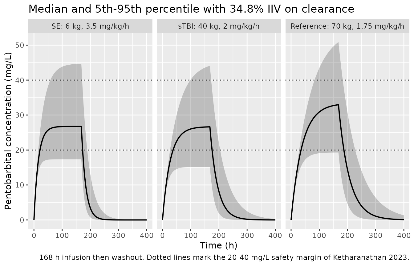

The 34.8% IIV on clearance alone spreads the steady-state concentration across roughly a two-fold range, which is the variability the paper’s covariate model was built to reduce.

PKNCA validation

sim_nca <- sim |>
  filter(!is.na(Cc)) |>
  select(id, time, Cc, arm)

# Guarantee a time = 0 row per (id, arm). This is an IV model with no dose
# before t = 0, so pre-dose Cc = 0 is correct.
sim_nca <- bind_rows(
  sim_nca,
  sim_nca |> distinct(id, arm) |> mutate(time = 0, Cc = 0)
) |>
  distinct(id, arm, time, .keep_all = TRUE) |>
  arrange(id, arm, time)

conc_obj <- PKNCA::PKNCAconc(
  sim_nca, Cc ~ time | arm + id,
  concu = "mg/L", timeu = "h"
)

dose_df <- events |>
  filter(evid == 1) |>
  select(id, time, amt, arm)

dose_obj <- PKNCA::PKNCAdose(dose_df, amt ~ time | arm + id, doseu = "mg")

intervals <- data.frame(
  start     = 0,
  end       = Inf,
  cmax      = TRUE,
  tmax      = TRUE,
  half.life = TRUE,
  auclast   = TRUE
)

nca_res <- PKNCA::pk.nca(PKNCA::PKNCAdata(conc_obj, dose_obj, intervals = intervals))

Comparison against published values

Ketharanathan 2023 does not report a conventional NCA table – the study is a continuous-infusion popPK analysis, so the published quantities that can be checked are the steady-state plateaus of the Figure 3 dosing scenarios and the cohort half-life quoted in the Discussion.

• Plateau concentrations. Sect. 3.5 states that rounding the infusion rates to 0.5 mg/kg/h steps made “the target concentrations ultimately reach 27 mg/L instead of the targeted 25 mg/L”, and Figure 3 shows the SE curves plateauing at about 27 mg/L and the sTBI curves at about 25 mg/L. With a 168 h infusion these plateaus are the observed Cmax.
• Half-life. The Discussion reports a pentobarbital half-life of 24.68 h, within the 5-50 h literature range. This is a cohort-level number with no weight attached, so it is compared here against the model’s own reference condition (70 kg, creatinine 36 umol/L, CRP at or below 70 mg/L).

published <- tribble(
  ~arm,                             ~cmax,      ~half.life,
  "SE: 6 kg, 3.5 mg/kg/h",           27.0,      NA_real_,
  "sTBI: 40 kg, 2 mg/kg/h",          25.0,      NA_real_,
  "Reference: 70 kg, 1.75 mg/kg/h",  NA_real_,  24.68
)

cmp <- nlmixr2lib::ncaComparisonTable(
  simulated     = nca_res,
  reference     = published,
  by            = "arm",
  units         = c(cmax = "mg/L", half.life = "h"),
  tolerance_pct = 20
)

knitr::kable(
  cmp,
  caption = "Simulated (median of 100 subjects per arm) vs. published values. * differs from reference by >20%.",
  align   = c("l", "l", "r", "r", "r")
)

Simulated (median of 100 subjects per arm) vs. published values. * differs from reference by >20%.

NCA parameter	arm	Reference	Simulated	% diff
Cmax (mg/L)	SE: 6 kg, 3.5 mg/kg/h	27	26.7	-0.9%
Cmax (mg/L)	sTBI: 40 kg, 2 mg/kg/h	25	26.6	+6.5%
Cmax (mg/L)	Reference: 70 kg, 1.75 mg/kg/h	—	33	—
t½ (h)	SE: 6 kg, 3.5 mg/kg/h	—	10.7	—
t½ (h)	sTBI: 40 kg, 2 mg/kg/h	—	18.8	—
t½ (h)	Reference: 70 kg, 1.75 mg/kg/h	24.7	26.8	+8.7%

The comparison is made on the individual-prediction scale (Cc), which is the scale of the published typical-value figures; the 7.22 mg/L additive residual error is an observation-level term and is not part of Figure 2-4.

The two plateau concentrations land within 6.5% of the published values and the reference-condition half-life is +8.7% against the cohort figure – no row exceeds the 20% tolerance. These arms carry the 34.8% IIV on clearance, so each simulated entry is the median over 100 subjects rather than a typical-value plateau; the corresponding typical-value steady states are 27.4 and 25.1 mg/L, which bracket the published 27 and 25 mg/L more tightly still.

The two dashed half-life rows have no published counterpart to compare against, and they are worth reading carefully. Because half-life in this model is log(2) * Vc / CL and the two allometric exponents differ (1 on volume, 0.75 on clearance), half-life is proportional to weight to the power 0.25 by construction. The single cohort figure of 24.68 h therefore cannot hold across a 3-87 kg population; it corresponds to a patient of about 46 kg at the model’s reference creatinine. The SE and sTBI arms are shorter still (10.7 h and 18.8 h) for a second reason: those arms replicate the Figure 3 scenario at creatinine 26 umol/L, which is below the 36 umol/L normalisation constant and so raises clearance by a factor of (26/36)^-0.919 = 1.35. The table below isolates the weight effect by holding creatinine at the model’s reference.

theta <- rxode2::rxode(readModelDb("Ketharanathan_2023_pentobarbital"))$theta
#> ℹ parameter labels from comments will be replaced by 'label()'

tibble(WT = c(3, 6, 10, 20, 40, 70, 87)) |>
  mutate(
    cl     = exp(theta[["lcl"]]) * (WT / 70)^0.75,
    vc     = exp(theta[["lvc"]]) * (WT / 70),
    `Typical half-life (h)` = round(log(2) * vc / cl, 1)
  ) |>
  transmute(
    "Body weight (kg)" = WT,
    "Typical CL (L/h)" = round(cl, 2),
    "Typical Vc (L)"   = round(vc, 1),
    `Typical half-life (h)`
  ) |>
  knitr::kable(
    caption = paste("Typical-value half-life across the cohort weight range at",
                    "the model's reference creatinine (36 umol/L) and",
                    "CRP <= 70 mg/L. Ketharanathan 2023 reports 24.68 h for the",
                    "cohort as a whole.")
  )

Typical-value half-life across the cohort weight range at the model’s reference creatinine (36 umol/L) and CRP <= 70 mg/L. Ketharanathan 2023 reports 24.68 h for the cohort as a whole.

Body weight (kg)	Typical CL (L/h)	Typical Vc (L)	Typical half-life (h)
3	0.34	6.1	12.5
6	0.57	12.2	14.8
10	0.83	20.3	16.9
20	1.40	40.6	20.0
40	2.36	81.1	23.8
70	3.59	142.0	27.4
87	4.23	176.5	28.9

Assumptions and deviations

• Residual error encoded as additive only. Sect. 3.2 states that “the residual error was described as an additive error, as the proportional error was estimated close to zero”, and Table 2 reports a single residual row in concentration units (“Additional (mg/L) 7.22”, 10% RSE, 6% shrinkage, bootstrap 95% CI 5.72-8.54 mg/L). The $ERROR block printed in the Supplementary Fig. 3 control stream is however

  W = IPRED+THETA(5)
  Y = IPRED+W*ERR(1)          with $SIGMA 1 FIX

  which would mean a residual SD of IPRED + 7.22 mg/L – a proportional term with a hardcoded coefficient of exactly 1, on top of the additive term. That reading is rejected here as a transcription artefact of the combined-error model the authors describe abandoning: deleting *THETA(6) from W = IPRED*THETA(6)+THETA(5) leaves exactly the printed line, and the $THETA block contains only five entries, so there is no sixth parameter for a proportional coefficient to have been estimated into. It is also numerically untenable – a residual SD of about 35 mg/L at the cohort median observation of 27.5 mg/L cannot be reconciled with the VPCs in Figure 1 or with the 6% shrinkage. The packaged model therefore uses Cc ~ add(addSd) with addSd = 7.22 mg/L, which matches every reported estimate. A user re-fitting this model should be aware of the discrepancy.

• CRP threshold comparison. The main-text equations apply the CRP term when CRP > 70 mg/L; the control stream uses IF(CRP.GE.70). The packaged model follows the control stream (>=). The two are numerically identical because (70/70)^-0.883 = 1 exactly.

• Two creatinine constants. 36 umol/L is the model’s creatinine normalisation constant (from the printed equation and the control stream); 26 umol/L is the value the authors chose as the input for the dosing simulations in Figs. 2, 3 and 4. The simulations in this vignette use 26 umol/L where they replicate those figures and 36 umol/L for the reference arm.

• Allometric exponents fixed. Both exponents are fixed() in ini(). Sect. 3.3 records that the clearance exponent was re-estimated during covariate analysis and that its confidence interval included 0.75, so the fixed value was retained; the exponents appear as hardcoded literals rather than $THETA entries in the control stream.

• No IIV on volume. Sect. 3.2: “Including an IIV resulted in a model improvement for CL only.” The packaged model has a single etalcl, so simulated volume is deterministic given weight.

• The 70 kg reference is an extrapolation. Cohort weights span 3-87 kg with a median of 10 kg, so the reported CL = 3.59 L/h/70 kg and Vc = 142 L/70 kg are allometric reference values rather than values observed in a typical study participant. The “Reference: 70 kg” arm used for the half-life comparison sits at the top of the observed weight range.

• Half-life is weight-dependent by construction. The differing allometric exponents (1 on volume, 0.75 on clearance) make half-life proportional to weight to the power 0.25, so the paper’s single cohort value of 24.68 h is reproduced only at about 46 kg. It is compared in the NCA table against the model’s reference condition only; the per-indication arms carry no published half-life. See the discussion and table above.

• Table 1 is typeset with a one-row label offset. In both the “Gender” and “Pentobarbital” blocks of Table 1 the category header carries a row of values while the last sub-row of the block (“Female”, “Max Infusion”) is blank, so the sub-row labels sit one line below the values they belong to. The sibling block pins the direction: read with the offset, the sTBI loading dose is 1 [0-20] mg/kg – exactly the per-protocol 1 mg/kg of Sect. 2.1 – and the min/max infusion rows reproduce the 0.5-10 and 0.05-5 mg/kg/h ranges quoted in Sect. 3.1; read without it, neither does. The population metadata therefore records 42% female (15 of 36), not 58%. Sex is not a covariate in the model (gender gave a dOFV of only 1.574 and was not retained), so this affects the metadata only and no simulated quantity.

• Covariates held constant over time. Creatinine and CRP were time-varying covariates in the original NONMEM dataset. The simulations here hold them constant per subject, matching the published figures, which do the same.

• Virtual cohort covariates are not sampled. Because every published figure fixes the covariates explicitly, the arms above reuse those exact values rather than sampling a demographic distribution. Only clearance carries between-subject variability.