Paracetamol and atorvastatin with semaglutide (Langeskov 2022)
Source:vignettes/articles/Langeskov_2022_semaglutide_ddi.Rmd
Langeskov_2022_semaglutide_ddi.RmdModel and source
Langeskov and Kristensen (2022) re-analysed two Novo Nordisk clinical pharmacology trials with population PK models to quantify how steady-state once-weekly subcutaneous semaglutide 1.0 mg, which slows gastric emptying, changes the absorption of two orally co-administered drugs. The two analyses were fitted separately (different trials, subjects and drugs), so the library carries them as two independent models that share this article.
- Citation: Langeskov EK, Kristensen K. Population pharmacokinetic of paracetamol and atorvastatin with co-administration of semaglutide. Pharmacol Res Perspect. 2022;10(4):e00962. doi:10.1002/prp2.962
- Paracetamol model: Two-compartment population PK model with first-order absorption and an absorption lag time for a single 1500 mg oral dose of paracetamol (solubilised in yoghurt) in healthy obese adults with and without steady-state once-weekly subcutaneous semaglutide 1.0 mg (Langeskov 2022). Semaglutide co-administration reduces the absorption rate constant by a fraction of 0.525 and body weight enters the apparent central volume linearly; proportional residual error.
- Atorvastatin model: Two-compartment population PK model with one transit compartment followed by first-order absorption for a single 40 mg oral dose of atorvastatin in healthy adults with and without steady-state once-weekly subcutaneous semaglutide 1.0 mg (Langeskov 2022). Semaglutide co-administration reduces ka and the transit rate constant ktr by fractions of 0.829 and 0.791; fixed allometric body-weight scaling (exponent 0.75 on clearances, 1 on volumes, 75 kg reference) and proportional residual error.
- Article: https://doi.org/10.1002/prp2.962
- Trial reports used for external checks: Hjerpsted et al. 2018 (paracetamol, https://doi.org/10.1111/dom.13120) and Hausner et al. 2017 (atorvastatin, https://doi.org/10.1007/s40262-017-0532-6).
Population
Paracetamol (trial NCT02079870). A randomised, double-blind, placebo-controlled two-period crossover in 30 healthy obese adults (BMI 30-45 kg/m^2). At the end of each 12-week period of semaglutide (escalated 0.25, 0.5 then 1.0 mg once weekly) or placebo, subjects received 1500 mg paracetamol solubilised in yoghurt, sampled at 0.25-5 h. The model was fitted to 503 samples from 29 subjects (20 male / 9 female), mean age 42 years (21-65), mean body weight 102 kg (81.5-121), mean BMI 33.2 kg/m^2 (Langeskov 2022 Table 1).
Atorvastatin (trial NCT02243098). An open-label one-sequence crossover in 31 healthy adults (BMI 20-30 kg/m^2). A single 40 mg atorvastatin dose was given before semaglutide was started and again in week 13 at semaglutide 1.0 mg steady state, sampled at 0.5-48 h. The model was fitted to 713 samples from 31 subjects (15 male / 16 female), mean age 45 years (25-55), mean body weight 75.4 kg (53.6-102), mean BMI 25.2 kg/m^2 (Table 1).
Both models were fitted in Phoenix NLME 8.1 (FOCE-ELS). The same
information is available programmatically from each model’s
population metadata, e.g.
readModelDb("Langeskov_2022_atorvastatin")()$population.
Source trace
Every ini() value carries an in-file comment pointing at
its source. The tables below collect them.
Paracetamol
(Langeskov_2022_paracetamol.R):
| Equation / parameter | Value | Source location |
|---|---|---|
lka (ka, placebo) |
log(9.4) 1/h | Table 2 |
e_conmed_semaglutide_ka |
0.525 | Table 2 ‘Theta kacovariate’; Section 3.2 |
lvc (V1/F at 102 kg) |
log(48.5) L | Table 2 |
e_wt_vc (linear, per kg) |
0.0312 | Table 2 ‘Theta V1/Fcovariate’; Section 3.2 |
lcl (CL/F) |
log(25.9) L/h | Table 2 |
lvp (V2/F) |
log(55.4) L | Table 2 |
lq (Cl2/F) |
log(199) L/h | Table 2 |
ltlag (Tlag) |
log(0.16) h | Table 2 |
etalka, etalvc, etalcl,
etalvp, etaltlag
|
0.514, 0.270, 0.0606, 0.0703, 0.0586 | Table 2 omega^2 |
propSd |
0.094 | Table 2 ‘Ceps’ (read as SD, see below) |
ka = tvka * (1 - theta * CONMED_SEMAGLUTIDE) |
n/a | Section 3.2 PML equation |
V1/F = tvV1/F * (1 + theta * (WT - MedianBW)) |
n/a | Section 3.2 PML equation |
| Two compartments, first-order absorption, lag | n/a | Figure 1; Section 3.1 |
Atorvastatin
(Langeskov_2022_atorvastatin.R):
| Equation / parameter | Value | Source location |
|---|---|---|
lka (ka, placebo) |
log(5.72) 1/h | Table 3 |
e_conmed_semaglutide_ka |
0.829 | Table 3 ‘Theta kacovariate’; Section 3.2 |
lktr (ktr, placebo) |
log(7.28) 1/h | Table 3 |
e_conmed_semaglutide_ktr |
0.791 | Table 3 ‘Theta ktrcovariate’; Section 3.2 |
lvc, lcl, lvp,
lq (75 kg) |
log(1843) L, log(620) L/h, log(4184) L, log(873) L/h | Table 3 (footnote a: 75 kg) |
e_wt_cl_q, e_wt_vc_vp
|
0.75, 1 (fixed) | Section 3.2 PML equations |
etalka, etalktr, etalvc,
etalcl, etalvp
|
2.03, 1.82, 0.625, 0.151, 0.111 | Table 3 omega^2 |
propSd |
0.322 | Table 3 ‘Ceps’ |
| dose -> transit -(ktr)-> absorption -(ka)-> central | n/a | Figure 2; Section 3.1 |
Virtual cohorts
Each treatment condition is simulated as its own arm of 200 virtual subjects (subject IDs are disjoint across arms). Body weight is drawn from a normal distribution truncated to the observed range: mean 102 kg, SD 10.5 kg for the paracetamol trial (Hjerpsted 2018 baseline SD) and mean 75.4 kg, SD 12 kg for the atorvastatin trial (SD not reported; chosen so that the observed range 53.6-102 kg spans roughly +/-2 SD).
set.seed(20220705)
rxode2::rxSetSeed(20220705)

draw_wt <- function(n, mean, sd, lo, hi) {
  wt <- rnorm(n, mean, sd)
  # Redraw out-of-range values until all fall in the observed range
  while (any(out <- wt < lo | wt > hi)) wt[out] <- rnorm(sum(out), mean, sd)
  wt
}

make_cohort <- function(n, dose, obs_times, sema, wt_mean, wt_sd, wt_lo, wt_hi,
                        id_offset = 0L) {
  subj <- tibble(
    id = id_offset + seq_len(n),
    WT = draw_wt(n, wt_mean, wt_sd, wt_lo, wt_hi),
    CONMED_SEMAGLUTIDE = sema,
    treatment = if (sema == 1) "Semaglutide" else "Placebo"
  )
  dose_rows <- subj |> mutate(time = 0, evid = 1L, amt = dose, cmt = "depot")
  obs_rows <- subj |>
    tidyr::crossing(time = obs_times) |>
    mutate(evid = 0L, amt = 0, cmt = "central")
  bind_rows(dose_rows, obs_rows) |> arrange(id, time, desc(evid))
}

para_times <- sort(unique(c(seq(0, 1, by = 0.05), seq(1.1, 5, by = 0.1), seq(5.5, 24, by = 0.5))))
ator_times <- sort(unique(c(seq(0, 4, by = 0.1), seq(4.5, 24, by = 0.5), seq(25, 96, by = 1))))

ev_para <- bind_rows(
  make_cohort(200, 1500, para_times, 0, 102, 10.5, 81.5, 121, id_offset = 0L),
  make_cohort(200, 1500, para_times, 1, 102, 10.5, 81.5, 121, id_offset = 200L)
)
ev_ator <- bind_rows(
  make_cohort(200, 40, ator_times, 0, 75.4, 12, 53.6, 102, id_offset = 0L),
  make_cohort(200, 40, ator_times, 1, 75.4, 12, 53.6, 102, id_offset = 200L)
)
stopifnot(
  !anyDuplicated(unique(ev_para[, c("id", "time", "evid")])),
  !anyDuplicated(unique(ev_ator[, c("id", "time", "evid")]))
)
Simulation
mod_para <- readModelDb("Langeskov_2022_paracetamol")
mod_ator <- readModelDb("Langeskov_2022_atorvastatin")

sim_para <- rxode2::rxSolve(mod_para, events = ev_para, keep = c("treatment", "WT")) |>
  as.data.frame() |>
  mutate(Cc_umol = Cc / 151.16 * 1000) # mg/L -> umol/L (MW 151.16 g/mol)
#> ℹ parameter labels from comments will be replaced by 'label()'
sim_ator <- rxode2::rxSolve(mod_ator, events = ev_ator, keep = c("treatment", "WT")) |>
  as.data.frame()
#> ℹ parameter labels from comments will be replaced by 'label()'
Replicate published figures
vpc_summary <- function(sim, conc, tmax) {
  sim |>
    filter(time > 0, time <= tmax) |>
    group_by(treatment, time) |>
    summarise(
      Q05 = quantile(.data[[conc]], 0.05),
      Q50 = quantile(.data[[conc]], 0.50),
      Q95 = quantile(.data[[conc]], 0.95),
      .groups = "drop"
    )
}

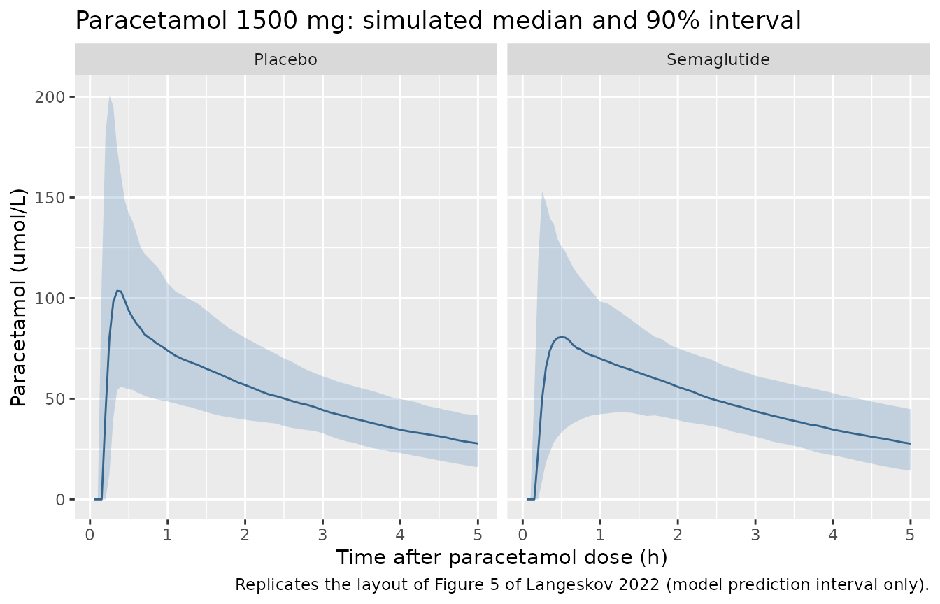
vpc_summary(sim_para, "Cc_umol", 5) |>
  ggplot(aes(time, Q50)) +
  geom_ribbon(aes(ymin = Q05, ymax = Q95), alpha = 0.25, fill = "steelblue") +
  geom_line(colour = "steelblue4") +
  facet_wrap(~treatment) +
  labs(
    x = "Time after paracetamol dose (h)", y = "Paracetamol (umol/L)",
    title = "Paracetamol 1500 mg: simulated median and 90% interval",
    caption = "Replicates the layout of Figure 5 of Langeskov 2022 (model prediction interval only)."
  )
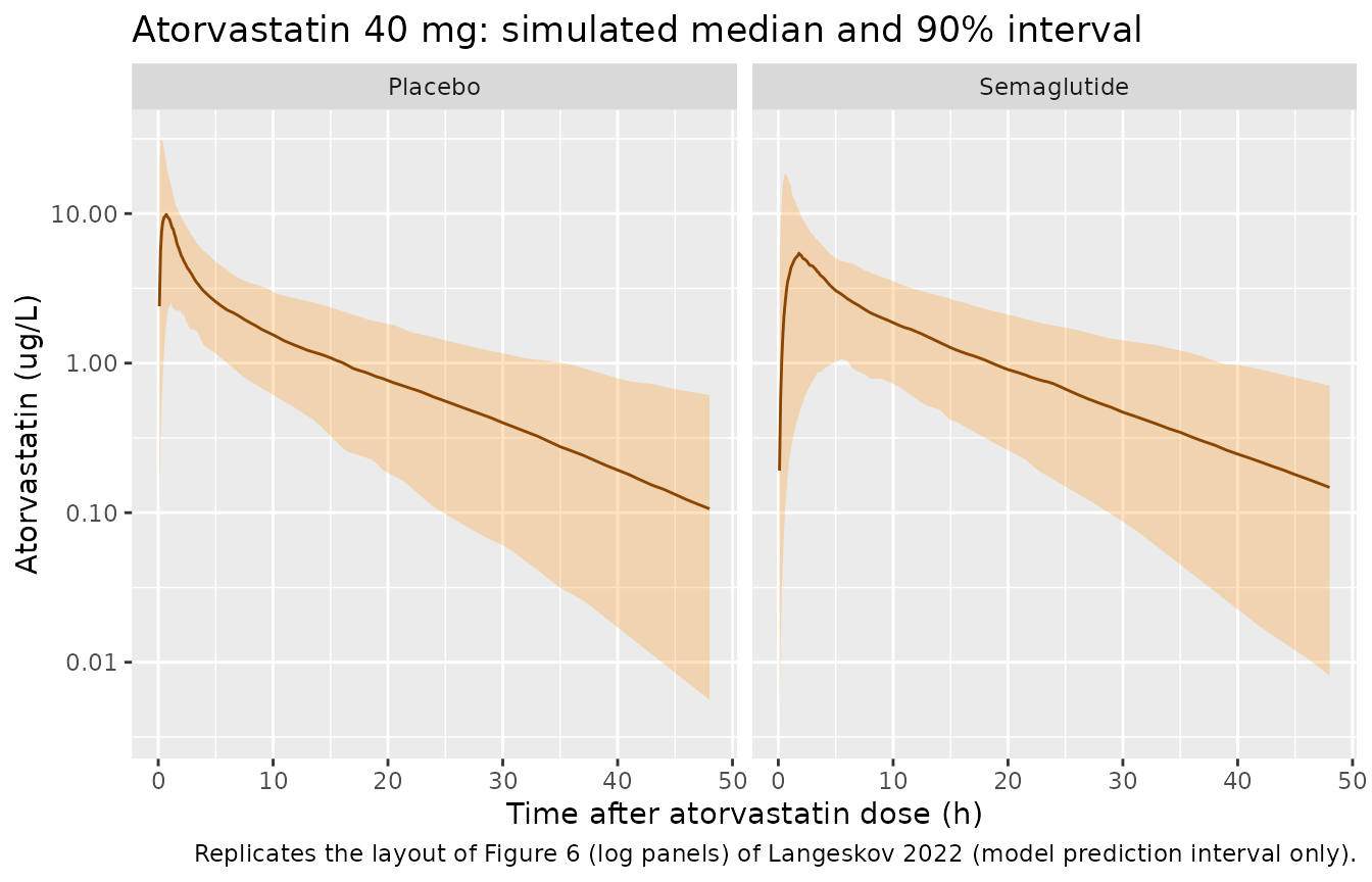
vpc_summary(sim_ator, "Cc", 48) |>
  ggplot(aes(time, Q50)) +
  geom_ribbon(aes(ymin = Q05, ymax = Q95), alpha = 0.25, fill = "darkorange") +
  geom_line(colour = "darkorange4") +
  facet_wrap(~treatment) +
  scale_y_log10() +
  labs(
    x = "Time after atorvastatin dose (h)", y = "Atorvastatin (ug/L)",
    title = "Atorvastatin 40 mg: simulated median and 90% interval",
    caption = "Replicates the layout of Figure 6 (log panels) of Langeskov 2022 (model prediction interval only)."
  )
Gastric retention and T50 (Figures 7 and 8)
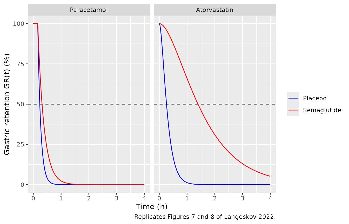
The paper derives a percent gastric retention curve GR(t) from the typical absorption parameters: the percentage of the dose still in the absorption compartments (for atorvastatin, the transit plus absorption compartments), and T50 as the time at which GR(t) reaches 50%. For paracetamol this is Equation 6, T50 = ln(2) / ka + Tlag. Here GR(t) is read directly off the model’s absorption states in a typical-value solve.
gr_events <- function(dose) {
  tt <- seq(0, 4, by = 0.001)
  bind_rows(
    tibble(id = 1:2, time = 0, evid = 1L, amt = dose, cmt = "depot"),
    tidyr::crossing(id = 1:2, time = tt) |> mutate(evid = 0L, amt = 0, cmt = "central")
  ) |>
    mutate(
      CONMED_SEMAGLUTIDE = id - 1L,
      treatment = if_else(id == 2L, "Semaglutide", "Placebo"),
      WT = 75
    ) |>
    arrange(id, time, desc(evid))
}

gr_para <- rxode2::rxSolve(rxode2::zeroRe(mod_para), events = gr_events(1500),
                           keep = "treatment", rtol = 1e-10, atol = 1e-12) |>
  as.data.frame() |>
  # Up to and including Tlag the dose has not yet entered `depot`; it is
  # still retained (at t = Tlag the observation precedes the lagged dose).
  mutate(GR = if_else(time <= 0.16, 100, 100 * depot / 1500), drug = "Paracetamol")
#> ℹ parameter labels from comments will be replaced by 'label()'
#> ℹ omega/sigma items treated as zero: 'etalka', 'etalvc', 'etalcl', 'etalvp', 'etaltlag'
#> Warning: multi-subject simulation without without 'omega'
gr_ator <- rxode2::rxSolve(rxode2::zeroRe(mod_ator), events = gr_events(40),
                           keep = "treatment", rtol = 1e-10, atol = 1e-12) |>
  as.data.frame() |>
  mutate(GR = 100 * (depot + transit1) / 40, drug = "Atorvastatin")
#> ℹ parameter labels from comments will be replaced by 'label()'
#> ℹ omega/sigma items treated as zero: 'etalka', 'etalktr', 'etalvc', 'etalcl', 'etalvp'
#> Warning: multi-subject simulation without without 'omega'

bind_rows(gr_para, gr_ator) |>
  mutate(drug = factor(drug, c("Paracetamol", "Atorvastatin"))) |>
  ggplot(aes(time, GR, colour = treatment)) +
  geom_line() +
  geom_hline(yintercept = 50, linetype = "dashed") +
  facet_wrap(~drug) +
  scale_colour_manual(values = c(Placebo = "blue", Semaglutide = "red")) +
  labs(
    x = "Time (h)", y = "Gastric retention GR(t) (%)", colour = NULL,
    caption = "Replicates Figures 7 and 8 of Langeskov 2022."
  )
t50 <- function(d) {
  d <- d[d$time > 0, ]
  i <- which(d$GR <= 50)[1]
  # Linear interpolation between the bracketing grid points
  d$time[i - 1] + (50 - d$GR[i - 1]) / (d$GR[i] - d$GR[i - 1]) * (d$time[i] - d$time[i - 1])
}
t50_tab <- bind_rows(gr_para, gr_ator) |>
  group_by(drug, treatment) |>
  group_modify(~ tibble(T50_h = t50(.x))) |>
  ungroup() |>
  mutate(
    T50_min = 60 * T50_h,
    published_min = c(16, 83, 0.23 * 60, 0.31 * 60)[match(paste(drug, treatment), c(
      "Atorvastatin Placebo", "Atorvastatin Semaglutide",
      "Paracetamol Placebo", "Paracetamol Semaglutide"
    ))]
  )

t50_tab |>
  dplyr::rename(
    "Drug" = drug, "Arm" = treatment, "T50 (h)" = T50_h,
    "T50 (min)" = T50_min, "Published T50 (min)" = published_min
  ) |>
knitr::kable(digits = 2, caption = "Typical-value T50 against Section 3.4 of Langeskov 2022.")| Drug | Arm | T50 (h) | T50 (min) | Published T50 (min) |
|---|---|---|---|---|
| Atorvastatin | Placebo | 0.26 | 15.67 | 16.0 |
| Atorvastatin | Semaglutide | 1.39 | 83.69 | 83.0 |
| Paracetamol | Placebo | 0.23 | 14.02 | 13.8 |
| Paracetamol | Semaglutide | 0.32 | 18.91 | 18.6 |
# Deterministic: typical-value solve at rtol 1e-10 on a 0.001 h grid.
# Paracetamol is printed to 0.01 h (0.23 / 0.31 h), atorvastatin to the minute.
para_t50 <- t50_tab$T50_h[t50_tab$drug == "Paracetamol"]
ator_t50 <- t50_tab$T50_min[t50_tab$drug == "Atorvastatin"]
stopifnot(
  length(para_t50) == 2L, length(ator_t50) == 2L,
  all(abs(para_t50 - c(0.23, 0.31)) < 0.006),
  all(abs(ator_t50 - c(16, 83)) < 1)
)
The model reproduces all four published T50 values: paracetamol 14 and 19 min (Equation 6 gives 0.234 and 0.315 h) and atorvastatin 16 and 83 min, i.e. the 67-minute semaglutide-induced delay in atorvastatin absorption reported in the Results.
PKNCA validation
run_nca <- function(sim, events, extra_intervals) {
  conc <- sim |>
    filter(!is.na(Cc)) |>
    select(id, time, Cc, treatment)
  conc <- bind_rows(conc, conc |> distinct(id, treatment) |> mutate(time = 0, Cc = 0)) |>
    distinct(id, treatment, time, .keep_all = TRUE) |>
    arrange(id, treatment, time)
  doses <- events |>
    filter(evid == 1) |>
    select(id, time, amt, treatment)
  intervals <- bind_rows(
    data.frame(start = 0, end = Inf, cmax = TRUE, tmax = TRUE, aucinf.obs = TRUE),
    extra_intervals
  ) |>
    # bind_rows() leaves NA in the flags a row does not set; PKNCA needs FALSE
    mutate(across(where(is.logical), ~ coalesce(.x, FALSE)))
  PKNCA::pk.nca(PKNCA::PKNCAdata(
    PKNCA::PKNCAconc(conc, Cc ~ time | treatment + id),
    PKNCA::PKNCAdose(doses, amt ~ time | treatment + id),
    intervals = intervals
  ))
}

nca_para <- run_nca(sim_para, ev_para, data.frame(start = 0, end = c(1, 5), aucint.last = TRUE))
nca_ator <- run_nca(sim_ator, ev_ator, data.frame(start = 0, end = 72, aucint.last = TRUE))

nca_summary <- function(nca) {
  as.data.frame(nca) |>
    filter(PPTESTCD %in% c("cmax", "tmax", "aucinf.obs", "aucint.last")) |>
    mutate(param = if_else(PPTESTCD == "aucint.last", paste0("auc0-", end), PPTESTCD)) |>
    group_by(treatment, param) |>
    summarise(
      value = if (first(PPTESTCD) == "tmax") median(PPORRES) else exp(mean(log(PPORRES))),
      .groups = "drop"
    )
}
para_sum <- nca_summary(nca_para)
ator_sum <- nca_summary(nca_ator)

bind_rows(
  para_sum |> mutate(drug = "Paracetamol (mg/L, h)"),
  ator_sum |> mutate(drug = "Atorvastatin (ug/L, h)")
) |>
  tidyr::pivot_wider(names_from = treatment, values_from = value) |>
  dplyr::rename("Drug (units)" = drug, "NCA parameter" = param) |>
knitr::kable(digits = 3, caption = "Simulated NCA: geometric means (median for tmax) per arm.")| NCA parameter | Drug (units) | Placebo | Semaglutide |
|---|---|---|---|
| auc0-1 | Paracetamol (mg/L, h) | 10.561 | 8.677 |
| auc0-5 | Paracetamol (mg/L, h) | 38.989 | 36.623 |
| aucinf.obs | Paracetamol (mg/L, h) | 59.415 | 57.557 |
| cmax | Paracetamol (mg/L, h) | 16.620 | 13.035 |
| tmax | Paracetamol (mg/L, h) | 0.350 | 0.500 |
| auc0-72 | Atorvastatin (ug/L, h) | 59.789 | 61.858 |
| aucinf.obs | Atorvastatin (ug/L, h) | 61.098 | 63.878 |
| cmax | Atorvastatin (ug/L, h) | 10.857 | 5.762 |
| tmax | Atorvastatin (ug/L, h) | 0.700 | 2.000 |
Mass balance: AUC does not depend on semaglutide
Semaglutide only slows absorption in both models, so AUC0-inf must equal dose / (CL/F) in both arms. A typical-value solve checks this identity.
typ_events <- function(dose, wt, tmax) {
  tt <- sort(unique(c(seq(0, 2, by = 0.01), seq(2, tmax, by = 0.1))))
  bind_rows(
    tibble(id = 1:2, time = 0, evid = 1L, amt = dose, cmt = "depot"),
    tidyr::crossing(id = 1:2, time = tt) |> mutate(evid = 0L, amt = 0, cmt = "central")
  ) |>
    mutate(CONMED_SEMAGLUTIDE = id - 1L, WT = wt) |>
    arrange(id, time, desc(evid))
}
trap <- function(x, y) sum(diff(x) * (head(y, -1) + tail(y, -1)) / 2)

typ_para <- rxode2::rxSolve(rxode2::zeroRe(mod_para), events = typ_events(1500, 102, 72),
                            rtol = 1e-10, atol = 1e-12) |> as.data.frame()
#> ℹ parameter labels from comments will be replaced by 'label()'
#> ℹ omega/sigma items treated as zero: 'etalka', 'etalvc', 'etalcl', 'etalvp', 'etaltlag'
#> Warning: multi-subject simulation without without 'omega'
typ_ator <- rxode2::rxSolve(rxode2::zeroRe(mod_ator), events = typ_events(40, 75, 480),
                            rtol = 1e-10, atol = 1e-12) |> as.data.frame()
#> ℹ parameter labels from comments will be replaced by 'label()'
#> ℹ omega/sigma items treated as zero: 'etalka', 'etalktr', 'etalvc', 'etalcl', 'etalvp'
#> Warning: multi-subject simulation without without 'omega'
auc_para <- tapply(seq_len(nrow(typ_para)), typ_para$id, function(i) trap(typ_para$time[i], typ_para$Cc[i]))
auc_ator <- tapply(seq_len(nrow(typ_ator)), typ_ator$id, function(i) trap(typ_ator$time[i], typ_ator$Cc[i]))
closed <- c(paracetamol = 1500 / 25.9, atorvastatin = 40 / 620 * 1000)
auc_tab <- tibble(
  drug = rep(names(closed), each = 2),
  treatment = rep(c("Placebo", "Semaglutide"), 2),
  AUC_solve = c(auc_para, auc_ator),
  AUC_closed_form = rep(closed, each = 2)
) |>
  mutate(rel_diff_pct = 100 * (AUC_solve / AUC_closed_form - 1))
auc_tab |>
  dplyr::rename(
    "Drug" = drug, "Arm" = treatment, "AUC (typical solve)" = AUC_solve,
    "Dose / (CL/F)" = AUC_closed_form, "Difference (%)" = rel_diff_pct
  ) |>
knitr::kable(digits = 3)| Drug | Arm | AUC (typical solve) | Dose / (CL/F) | Difference (%) |
|---|---|---|---|---|
| paracetamol | Placebo | 57.914 | 57.915 | -0.001 |
| paracetamol | Semaglutide | 57.916 | 57.915 | 0.001 |
| atorvastatin | Placebo | 64.519 | 64.516 | 0.005 |
| atorvastatin | Semaglutide | 64.516 | 64.516 | 0.000 |
Comparison against the trial reports
Langeskov 2022 reports no NCA of its own. The two trial reports give the semaglutide / placebo ratios of the NCA endpoints, which the simulated arms can be compared against.
ratio <- function(s, p) {
  s$value[s$treatment == "Semaglutide" & s$param == p] /
    s$value[s$treatment == "Placebo" & s$param == p]
}
tmax_med <- function(s, arm) s$value[s$treatment == arm & s$param == "tmax"]

ratio_tab <- tibble::tribble(
  ~drug, ~endpoint, ~simulated, ~published, ~published_ci, ~source,
  "Atorvastatin", "AUC ratio", ratio(ator_sum, "auc0-72"), 1.02, "0.93-1.12", "Hausner 2017 Table 2",
  "Atorvastatin", "Cmax ratio", ratio(ator_sum, "cmax"), 0.62, "0.47-0.82", "Hausner 2017 Table 2",
  "Atorvastatin", "Median tmax, placebo (h)", tmax_med(ator_sum, "Placebo"), 0.7, "", "Hausner 2017 Results",
  "Atorvastatin", "Median tmax, semaglutide (h)", tmax_med(ator_sum, "Semaglutide"), 2.0, "", "Hausner 2017 Results",
  "Paracetamol", "AUC0-5h ratio", ratio(para_sum, "auc0-5"), 0.94, "0.88-1.01", "Hjerpsted 2018 Section 3.4",
  "Paracetamol", "AUC0-1h ratio", ratio(para_sum, "auc0-1"), 0.73, "0.61-0.87", "Hjerpsted 2018 Section 3.4"
)
ratio_tab |>
  dplyr::rename(
    "Drug" = drug, "Endpoint" = endpoint, "Simulated" = simulated,
    "Published" = published, "Published CI" = published_ci, "Source" = source
  ) |>
knitr::kable(digits = 2, caption = "Semaglutide / placebo NCA ratios: simulated arms (200 each) vs the trial reports.")| Drug | Endpoint | Simulated | Published | Published CI | Source |
|---|---|---|---|---|---|
| Atorvastatin | AUC ratio | 1.03 | 1.02 | 0.93-1.12 | Hausner 2017 Table 2 |
| Atorvastatin | Cmax ratio | 0.53 | 0.62 | 0.47-0.82 | Hausner 2017 Table 2 |
| Atorvastatin | Median tmax, placebo (h) | 0.70 | 0.70 | Hausner 2017 Results | |
| Atorvastatin | Median tmax, semaglutide (h) | 2.00 | 2.00 | Hausner 2017 Results | |
| Paracetamol | AUC0-5h ratio | 0.94 | 0.94 | 0.88-1.01 | Hjerpsted 2018 Section 3.4 |
| Paracetamol | AUC0-1h ratio | 0.82 | 0.73 | 0.61-0.87 | Hjerpsted 2018 Section 3.4 |
sim_ratio <- setNames(ratio_tab$simulated, paste(ratio_tab$drug, ratio_tab$endpoint))
stopifnot(
  # Exposure is unchanged by semaglutide in both models (CL/F has no
  # semaglutide effect); between-arm noise in the geometric-mean ratio is
  # roughly 3-4% (1 SE) at 200 per arm, so 15% is about 4 SE.
  abs(log(sim_ratio[["Atorvastatin AUC ratio"]])) < log(1.15),
  abs(log(sim_ratio[["Paracetamol AUC0-5h ratio"]])) < log(1.15),
  # The atorvastatin Cmax ratio sits inside the published 90% CI; the typical
  # value is 0.53 and the cohort noise is about 6%.
  sim_ratio[["Atorvastatin Cmax ratio"]] > 0.4,
  sim_ratio[["Atorvastatin Cmax ratio"]] < 0.75
)
The atorvastatin model reproduces the trial’s findings: unchanged AUC, a Cmax lowered by roughly half (published 38%, 90% CI 23-53%), and median tmax delayed from 0.7 h to 2 h. For paracetamol the overall exposure is unchanged as observed (AUC0-5h ratio about 0.94). The first-hour effect is weaker in the model than in the trial’s NCA: the simulated AUC0-1h ratio of about 0.8 lies inside the published 95% CI but above its point estimate of 0.73. The model places the whole semaglutide effect on ka (53% lower), with a 0.16 h lag shared by both arms, which delays T50 by only 5 minutes; the authors draw the same conclusion in their Discussion. The AUC0-1h ratio is reported but not gated.
Assumptions and deviations
-
Residual error scale. Tables 2 and 3 print the
residual row as ‘Ceps’ and the footnote calls Ceps sigma^2. Phoenix NLME
reports CEps as the standard deviation of epsilon, and the paracetamol
observed-vs-IPRED panel (Figure 3A) shows a scatter of about +/-10%
around the line of identity, which matches an SD of 9.4% and not the 31%
that a variance reading (sqrt(0.094)) implies. Both models therefore use
propSd= the printed value (0.094 and 0.322). - Paracetamol weight centring. The PML equation centres the linear weight effect on V1/F at ‘MedianBW’, which the paper does not print. The cohort mean of 102 kg (Table 1) is used. The linear form reaches V1/F = 0 at 70 kg, so the paracetamol model should not be used below the studied 81.5-121 kg range.
- Atorvastatin allometry. The PML examples show exponent 0.75 on CL/F and 1 on V1/F; the text says all four disposition parameters were scaled, so Cl2/F takes 0.75 and V2/F takes 1. The reference weight of 75 kg comes from the Table 3 footnote (‘For an individual of 75 kg’).
-
Compartment names for atorvastatin. Figure 2 names
the dose-receiving compartment ‘transit’ and the next one ‘absorption’.
In the library model the dose enters
depot(the paper’s transit compartment, emptied at rate ktr) andtransit1is the paper’s absorption compartment (emptied at rate ka), so doses use the conventionalcmt = "depot". -
Semaglutide indicator. The source data-set column
was named
placebobut was coded 1 for semaglutide co-administration (Section 3.2). It is carried asCONMED_SEMAGLUTIDEwith the same coding. - Inconsistent percentages in the paper. Table 3 and Section 3.2 give fractional reductions of 0.829 (ka) and 0.791 (ktr), i.e. 83% and 79%, and ka 5.72 -> 0.986 1/h; the Abstract and Discussion instead quote 72% and 91% and ka 4.8 -> 1.3 1/h, apparently from an earlier model. The Table 3 values are used; they reproduce the published T50 values of 16 and 83 minutes. The Figure 8 caption gives the atorvastatin placebo T50 as 0.22 h (13 min) where the Results give 16 min; the model gives 15.7 min.
- Virtual cohorts. Body-weight SD for the atorvastatin trial is not reported (12 kg assumed). Each condition is simulated as a separate arm rather than as a crossover; the models carry no inter-occasion variability, so a crossover would differ only in pairing.
- Errata. No correction notice for Langeskov 2022 was found in Europe PMC as of 2026-10-02.