Salbutamol (Marques 2024)
Source:vignettes/articles/Marques_2024_salbutamol.Rmd
Marques_2024_salbutamol.RmdModel and source
- Citation: Marques L, Vale N. Toward Personalized Salbutamol Therapy: Validating Virtual Patient-Derived Population Pharmacokinetic Model with Real-World Data. Pharmaceutics. 2024;16(7):881. doi:10.3390/pharmaceutics16070881. Parameters from Table 4 (final model refitted to the GlaxoSmithKline clinical dataset, NCT01984086 Part A Treatment A, accessed via Vivli).
- Article: https://doi.org/10.3390/pharmaceutics16070881
- Supplementary material: https://www.mdpi.com/article/10.3390/pharmaceutics16070881/s1
Marques and Vale generated a synthetic cohort of 32 virtual patients from GastroPlus PBPK models of a 600 ug salbutamol dry-powder-inhaler dose, fitted a population PK model to that synthetic cohort (their Table 3), and then refitted the same structure to a real clinical dataset – GlaxoSmithKline study NCT01984086 Part A Treatment A, 30 healthy volunteers given the same 600 ug UD-DPI dose, accessed through Vivli – as an external validation (their Table 4).
This package entry encodes Table 4 only, and encodes it as a one-compartment model. Both of those are deliberate departures from the paper’s own presentation, and both are forced by arithmetic in the paper. The “What this model is not” section below states the reasoning in full; read it before using the model.
#> ℹ parameter labels from comments will be replaced by 'label()'One-compartment population PK model for inhaled salbutamol (600 ug single dose, unit-dose dry-powder inhaler) in healthy adults, with first-order absorption, no lag time, and linear elimination. Encodes the EXTERNAL-VALIDATION fit to real clinical data (GSK study NCT01984086, n = 30; Marques 2024 Table 4) – NOT the paper’s headline virtual-patient model (Table 3), whose central volume of 0.02e-9 L is not solvable at any ODE tolerance and overshoots the paper’s own observed Cmax by four orders of magnitude. The authors declare a two-compartment structure, but their clinical-data fit returned Q = 1.30e-7 L/h and V2 = 0 exactly, both with relative standard errors above 1e6 percent (the authors’ own footnote calls this overparametrization); the peripheral compartment therefore carries no flux and k21 = Q/V2 is undefined, so the model is encoded honestly as one compartment. No covariate effects are encoded: the paper reports which covariates were significant but publishes no coefficients, functional forms, or centering values anywhere in the article or its supplement (see covariatesDataExcluded and the vignette Errata).
Population
The population is the clinical cohort of Marques 2024 Table 1, column “Clinical Study Patients (n = 30)”: healthy nonsmoking volunteers aged 18-65 years (mean 26.8, SD 4.8), weight >= 50 kg (mean 78.9, SD 17.6 kg), BMI 19.0-34.0 kg/m^2 (mean 24.7, SD 3.8), height 177.8 cm (SD 9.5), 8 female / 22 male, 90% White, 7% Mixed race and 3% American Indian or Alaskan Native. Each subject received a single 600 ug dose (3 x 200 ug blisters) by unit-dose dry powder inhaler, with plasma sampling at 0, 0.08, 0.17, 0.33, 0.50, 0.75, 1, 1.5, 2, 4, 6, 8, 10 and 12 h.
Note that this is not the 32-subject virtual cohort (Table 1, first column; Supplementary Table S1) that produced the paper’s Table 3 model. The two populations differ substantially – the virtual cohort is 38% American Indian / Alaskan Native and 62% East Asian, spans ages 5 to 65, and has a mean weight of 50.4 kg.
local({
  fbody <- body(readModelDb("Marques_2024_salbutamol"))
  meta_env <- new.env()
  for (stmt in as.list(fbody)[-1]) {
    if (is.call(stmt) && length(stmt) >= 1 &&
        identical(stmt[[1]], as.name("<-"))) {
      eval(stmt, envir = meta_env)
    } else {
      break
    }
  }
  cat("Population:\n")
  str(meta_env$population, max.level = 1)
  cat("\nCovariates screened by the authors but NOT encodable:\n")
  str(meta_env$covariatesDataExcluded, max.level = 1)
})
#> Population:
#> List of 13
#>  $ species       : chr "human"
#>  $ n_subjects    : num 30
#>  $ n_studies     : num 1
#>  $ age_range     : chr "18-65 years (eligibility criterion)"
#>  $ age_median    : chr "26.8 years (mean, SD 4.8; Table 1)"
#>  $ weight_range  : chr ">= 50 kg (eligibility criterion); BMI 19.0-34.0 kg/m^2"
#>  $ weight_median : chr "78.9 kg (mean, SD 17.6; Table 1)"
#>  $ sex_female_pct: num 26.7
#>  $ race_ethnicity: Named num [1:4] 90 7 3 0
#>   ..- attr(*, "names")= chr [1:4] "White" "Multi" "AmericanIndianOrAlaskanNative" "Asian"
#>  $ disease_state : chr "Healthy nonsmoking volunteers (no asthma)"
#>  $ dose_range    : chr "600 ug salbutamol (as sulfate) as a single dose: 3 x 200 ug blisters inhaled via unit-dose dry-powder inhaler (UD-DPI)"
#>  $ regions       : chr NA
#>  $ notes         : chr "GlaxoSmithKline study NCT01984086, Part A Treatment A, accessed through Vivli. Open-label, randomized, crossove"| __truncated__
#>
#> Covariates screened by the authors but NOT encodable:
#> List of 5
#>  $ AGE                 :List of 6
#>  $ WT                  :List of 6
#>  $ HT                  :List of 6
#>  $ SEXF                :List of 6
#>  $ RACE_ASIAN_NORTHEAST:List of 6
Source trace
Every ini() value and every model()
equation, with its origin. The same provenance is recorded as in-file
comments in
inst/modeldb/specificDrugs/Marques_2024_salbutamol.R.
| Parameter / equation | Value | Source location |
|---|---|---|
lka (absorption rate constant) |
log(13.55) 1/h |
Table 4, Fixed Effects: ka = 13.55 1/h (RSE 18.0%) |
lcl (apparent clearance) |
log(34.93) L/h |
Table 4, Fixed Effects: Cl = 34.93 L/h (RSE 16.6%) |
lvc (apparent central volume) |
log(162.93) L |
Table 4, Fixed Effects: V1 = 162.93 L (RSE 22.6%) |
etalka |
0.7921 |
Table 4, Random Effects: IIV(ka) = 0.89 (RSE 15.4%); variance = 0.89^2 |
etalcl |
0.2601 |
Table 4, Random Effects: IIV(Cl) = 0.51 (RSE 13.3%); variance = 0.51^2 |
etalvc |
0.1681 |
Table 4, Random Effects: IIV(V1) = 0.41 (RSE 13.4%); variance = 0.41^2 |
cov(etalcl, etalvc) |
0.192372 |
Table 4, Correlation: V1 and Cl = 0.92 (RSE 3.98); 0.92 x 0.51 x 0.41 |
addSd |
fixed(0) |
Section 2.3 declares the Monolix “combined 1” error model; the coefficient is never published (see Errata) |
propSd |
fixed(0) |
Section 2.3 declares the Monolix “combined 1” error model; the coefficient is never published (see Errata) |
d/dt(depot) |
-ka * depot |
Section 3.3: first-order absorption, no delay |
d/dt(central) |
ka * depot - kel * central |
Section 3.3: linear elimination |
kel <- cl / vc |
derived | standard one-compartment micro-constant |
Cc <- central / vc |
derived | dose in ug over volume in L gives ug/L = ng/mL |
(omitted) lq, lvp
|
– | Table 4 gives Q = 1.30e-7 L/h and V2 = 0; not encodable (see below) |
Monolix reports random effects as omega, the
standard deviation of the log-normally distributed
random effect. nlmixr2’s ini() takes
variances, so each published value is squared above. The
Correlation rows of Table 4 are correlation coefficients,
converted to a covariance by multiplying by both standard
deviations.
What this model is not
Three defects in the source constrain what can honestly be packaged. Each is stated here with the arithmetic that establishes it, so a reader can check the reasoning against the paper rather than take it on trust.
1. The paper’s headline model (Table 3) is not solvable
Table 3 – the fit to the 32 virtual patients, which is the paper’s
primary result – reports V1 = 0.02 x 10^-9 L, i.e. 2 x 10^-11 L, with an
RSE printed as NaN (“infinitely large standard error”, per
the table footnote).
t3 <- list(ka = 3.71, cl = 24.33, v1 = 0.02e-9, q = 10.59, v2 = 0.66e-2)
tibble::tibble(
  Quantity = c("kel = Cl / V1 (1/h)",
               "k12 = Q / V1 (1/h)",
               "Vss = V1 + V2 (L)",
               "Upper bound on Cmax = Dose / Vss (ug/mL)",
               "Paper's own observed virtual Cmax, Table 2 (ug/mL)",
               "Overshoot factor"),
  Value = c(
    formatC(t3$cl / t3$v1, format = "e", digits = 2),
    formatC(t3$q  / t3$v1, format = "e", digits = 2),
    formatC(t3$v1 + t3$v2, format = "f", digits = 5),
    formatC((600 / (t3$v1 + t3$v2)) / 1000, format = "f", digits = 2),
    "0.00650",
    formatC(((600 / (t3$v1 + t3$v2)) / 1000) / 0.00650, format = "e", digits = 2)
  )
) |>
knitr::kable(caption = "Table 3 of Marques 2024 is internally self-falsifying.")| Quantity | Value |
|---|---|
| kel = Cl / V1 (1/h) | 1.22e+12 |
| k12 = Q / V1 (1/h) | 5.30e+11 |
| Vss = V1 + V2 (L) | 0.00660 |
| Upper bound on Cmax = Dose / Vss (ug/mL) | 90.91 |
| Paper’s own observed virtual Cmax, Table 2 (ug/mL) | 0.00650 |
| Overshoot factor | 1.40e+04 |
Elimination and distribution rate constants of order 1011-1012 per hour make the ODE system infinitely stiff: it is not solvable at any tolerance. Worse, the most generous conceivable exposure – the entire 600 ug dose placed instantaneously into the total steady-state volume, with no absorption loss and no elimination – exceeds the paper’s own observed virtual Cmax by four orders of magnitude. No bioavailability, dose-unit or volume-unit reading reconciles this; it would require F = 7 x 10^-5.
Nor is it a recoverable units slip. Table 5 reports the individual empirical Bayes estimates for the same virtual population, stratified by subgroup. Pooling its Gender rows over the 14 female and 18 male virtual subjects of Table 1 gives a whole-cohort geometric mean per parameter, which can be compared directly against Table 3:
# Marques 2024 Table 5, Gender rows. Note Table 5 is in mL and mL/h whereas
# Table 3 is in L and L/h; the conversion is applied here.
t5 <- tibble::tribble(
  ~param, ~female,   ~male,     ~to_litres,
  "ka",    0.00610,  0.00890,   1,        # 1/h, no volume to convert
  "Cl",    5.07,     7.37,      1e-3,     # mL/h -> L/h
  "V1",    0.310e-4, 0.660e-4,  1e-3,     # mL   -> L
  "Q",     0.590e-7, 0.210e-6,  1e-3,     # mL/h -> L/h
  "V2",    0.00500,  0.300,     1e-3      # mL   -> L
)

pooled <- t5 |>
  dplyr::mutate(
    # n-weighted geometric mean over the 14 female / 18 male virtual subjects
    table5 = exp((14 * log(female) + 18 * log(male)) / 32) * to_litres,
    table3 = c(t3$ka, t3$cl, t3$v1, t3$q, t3$v2),
    ratio  = table3 / table5
  )

pooled |>
  dplyr::transmute(
    Parameter = param,
    `Table 5 pooled` = formatC(table5, format = "e", digits = 2),
    `Table 3`        = formatC(table3, format = "e", digits = 2),
    `Table 3 / Table 5` = formatC(ratio, format = "e", digits = 2)
  ) |>
knitr::kable(caption = "Table 3 and Table 5 describe the same 32 virtual subjects but disagree by parameter-specific factors spanning 14 orders of magnitude.")| Parameter | Table 5 pooled | Table 3 | Table 3 / Table 5 |
|---|---|---|---|
| ka | 7.54e-03 | 3.71e+00 | 4.92e+02 |
| Cl | 6.26e-03 | 2.43e+01 | 3.89e+03 |
| V1 | 4.74e-08 | 2.00e-11 | 4.22e-04 |
| Q | 1.21e-10 | 1.06e+01 | 8.79e+10 |
| V2 | 5.00e-05 | 6.60e-03 | 1.32e+02 |
The ratios run from 4 x 10^-4 (V1) to 9 x 10^10 (Q). There is no single scale factor – no unit slip, no dose-normalisation, no per-kg convention – that maps one table onto the other.
Table 3 is therefore not packaged in any form.
2. The covariate layer is entirely unreported
The paper’s title, abstract, and Section 3.4 foreground a covariate model: age on Cl and Q; gender on ka and Cl; race on Cl; weight on Cl, Q and V2. No coefficient, functional form, reference value or centering constant for any of these appears anywhere in the article or in Supplementary Tables S1-S2. Table 5 is a descriptive stratification of individual EBE parameters into subgroups, not a set of covariate effects, and it is reported in units irreconcilable with Table 3.
The screened covariates are recorded in the model file’s
covariatesDataExcluded metadata (printed above) so the
paper’s claim is preserved, but none can be encoded. Nothing here is a
substitute for the missing coefficients.
3. Table 4’s peripheral compartment collapsed to zero
The authors describe Table 4 as a two-compartment fit. Their own estimates say otherwise: Q = 1.30 x 10^-7 L/h (RSE 2.83 x 10^6 %) and V2 = 0 exactly (RSE 1.35 x 10^7 %), both carrying the table footnote “values are very large standard errors, potentially suggesting an overparametrization of the model”.
V2 = 0 makes the return micro-constant k21 = Q / V2 a
division of zero by zero – undefined, not small. And Q is eight orders
of magnitude below Cl, so even treating V2 as merely tiny, the
peripheral compartment exchanges no material amount of drug. There is no
honest two-compartment encoding of Table 4; it is a one-compartment
model in the authors’ own numbers, and it is packaged as one.
Model behaviour
mod <- readModelDb("Marques_2024_salbutamol")

ka <- 13.55; cl <- 34.93; vc <- 162.93
kel <- cl / vc
tmax_analytic <- log(ka / kel) / (ka - kel)
cmax_analytic <- (600 / vc) * (kel / ka)^(kel / (ka - kel))

tibble::tibble(
  Quantity = c("kel = Cl / Vc (1/h)", "Terminal half-life (h)",
               "Analytic Tmax (h)", "Analytic Cmax (ng/mL)",
               "AUC(0-inf) = Dose / Cl (ng*h/mL)"),
  Value = round(c(kel, log(2) / kel, tmax_analytic, cmax_analytic, 600 / cl), 4)
) |>
knitr::kable(caption = "Typical-value quantities implied by Table 4, reduced to one compartment.")| Quantity | Value |
|---|---|
| kel = Cl / Vc (1/h) | 0.2144 |
| Terminal half-life (h) | 3.2332 |
| Analytic Tmax (h) | 0.3109 |
| Analytic Cmax (ng/mL) | 3.4451 |
| AUC(0-inf) = Dose / Cl (ng*h/mL) | 17.1772 |
The exact-Tmax gate
Tmax is the one published clinical NCA statistic that is independent of the concentration scale, and it is therefore the strongest available check that the reduced model reproduces the source. Marques 2024 Table 2 reports an observed clinical Tmax of 0.310 h; the model implies 0.3109 h.
ev_typ <- rxode2::et(amt = 600, cmt = "depot") |>
  rxode2::et(seq(0, 12, by = 0.001), cmt = "central")

sim_typ <- rxode2::rxSolve(rxode2::zeroRe(mod), ev_typ, omega = NA,
                           returnType = "data.frame")
#> ℹ parameter labels from comments will be replaced by 'label()'
tmax_sim <- sim_typ$time[which.max(sim_typ$Cc)]

stopifnot(abs(tmax_sim - 0.310) < 0.01)

tibble::tibble(
  Source = c("Marques 2024 Table 2, clinical dataset (observed)",
             "This model, solved on a 0.001 h grid",
             "This model, closed form ln(ka/kel)/(ka-kel)"),
  `Tmax (h)` = c(0.310, tmax_sim, tmax_analytic)
) |>
knitr::kable(digits = 4, caption = "Tmax reproduces the published clinical value to three significant figures.")| Source | Tmax (h) |
|---|---|
| Marques 2024 Table 2, clinical dataset (observed) | 0.3100 |
| This model, solved on a 0.001 h grid | 0.3110 |
| This model, closed form ln(ka/kel)/(ka-kel) | 0.3109 |
Virtual cohort and simulation
The model carries no covariates, so the cohort is defined entirely by the inter-individual random effects of Table 4. We simulate 200 subjects – ample for a prediction interval, and well inside the vignette time budget – on the paper’s own sampling grid plus a denser grid for the profile figure.
set.seed(2026L)
n_sub <- 200L

paper_times <- c(0, 0.08, 0.17, 0.33, 0.50, 0.75, 1, 1.5, 2, 4, 6, 8, 10, 12)
# Rounded so the paper's sample times are bit-identical between the two grids
# and the NCA join below cannot miss a record to floating-point drift.
dense_times <- sort(unique(round(c(paper_times, seq(0, 12, by = 0.05)), 3)))

doses <- tibble::tibble(
  id = seq_len(n_sub), time = 0, evid = 1L, amt = 600,
  cmt = "depot", treatment = "600 ug UD-DPI single dose"
)

obs <- tidyr::expand_grid(id = seq_len(n_sub), time = dense_times) |>
  dplyr::transmute(id, time, evid = 0L, amt = NA_real_,
                   cmt = "central", treatment = "600 ug UD-DPI single dose")

events <- dplyr::bind_rows(doses, obs) |>
  dplyr::arrange(id, time, dplyr::desc(evid))

sim <- rxode2::rxSolve(mod, events = events, keep = "treatment") |>
  as.data.frame()
#> ℹ parameter labels from comments will be replaced by 'label()'

nrow(sim)
#> [1] 48800
Because the residual-error coefficients are unpublished and therefore
fixed at zero, the sim column equals the individual
prediction Cc; the spread below is pure inter-individual
variability.
vpc <- sim |>
  # drop only the pre-dose record, which is identically zero and cannot be
  # drawn on a log axis; the NCA below keeps it
  dplyr::filter(!dplyr::near(time, 0)) |>
  dplyr::group_by(time) |>
  dplyr::summarise(
    med = median(Cc),
    lo  = quantile(Cc, 0.05),
    hi  = quantile(Cc, 0.95),
    .groups = "drop"
  )

ggplot(vpc, aes(time, med)) +
  geom_ribbon(aes(ymin = lo, ymax = hi), alpha = 0.18, fill = "steelblue") +
  geom_line(colour = "firebrick", linewidth = 0.8) +
  geom_hline(yintercept = 0.160, linetype = "dashed", colour = "grey35") +
  annotate("point", x = 0.310, y = 0.160, colour = "grey20", size = 2) +
  scale_y_log10() +
  labs(x = "Time (h)", y = "Plasma salbutamol (ng/mL)",
       title = "Single 600 ug salbutamol UD-DPI dose",
       caption = "Red = median, blue ribbon = 90% PI. Grey point = Table 2 clinical geometric-mean (Tmax, Cmax).") +
  theme_minimal()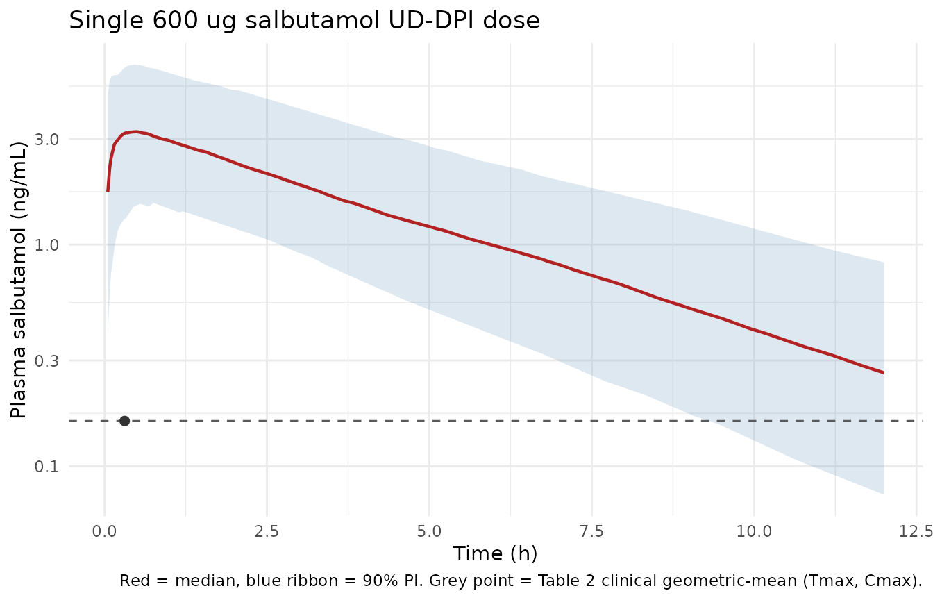
Simulated plasma salbutamol after a single 600 ug UD-DPI dose, N = 200. Solid line = median; ribbon = 90% prediction interval. Comparable to Figure 7 of Marques 2024 (VPC of the clinical dataset). The dashed line and point mark the geometric-mean Cmax and Tmax reported for the clinical dataset in Table 2.
PKNCA validation
NCA is run on the paper’s own sampling grid, so the simulated statistics are computed from the same information the authors’ NCA had. The time-zero record is retained deliberately: dropping it makes PKNCA warn that the AUC interval starts before the first measurement.
sim_nca <- sim |>
  dplyr::filter(!is.na(Cc)) |>
  dplyr::inner_join(tibble::tibble(time = round(paper_times, 3)), by = "time") |>
  dplyr::select(id, time, Cc, treatment)

# The time = 0 record must survive to PKNCA, or every subject warns that the
# AUC interval starts before the first measurement.
stopifnot(0 %in% sim_nca$time,
          nrow(sim_nca) == n_sub * length(paper_times))

dose_df <- events |>
  dplyr::filter(evid == 1L) |>
  dplyr::select(id, time, amt, treatment)

conc_obj <- PKNCA::PKNCAconc(sim_nca, Cc ~ time | treatment + id,
                             concu = "ng/mL", timeu = "h")
dose_obj <- PKNCA::PKNCAdose(dose_df, amt ~ time | treatment + id,
                             doseu = "ug")

intervals <- data.frame(
  start      = 0,
  end        = Inf,
  cmax       = TRUE,
  tmax       = TRUE,
  auclast    = TRUE,
  aucinf.obs = TRUE,
  half.life  = TRUE
)

nca_res <- PKNCA::pk.nca(PKNCA::PKNCAdata(conc_obj, dose_obj,
                                          intervals = intervals))
summary(nca_res)
#>  Interval Start Interval End                 treatment   N AUClast (h*ng/mL)
#>               0          Inf 600 ug UD-DPI single dose 200       15.1 [51.9]
#>  Cmax (ng/mL)             Tmax (h) Half-life (h) AUCinf,obs (h*ng/mL)
#>   3.28 [45.2] 0.330 [0.0800, 2.00]  3.24 [0.684]          16.4 [55.1]
#>
#> Caption: AUClast, Cmax, AUCinf,obs: geometric mean and geometric coefficient of variation; Tmax: median and range; Half-life: arithmetic mean and standard deviation; N: number of subjects
Comparison against the published NCA
Table 2 of Marques 2024 reports the clinical dataset’s NCA as
geometric means in ug/mL and ugh/mL; the values below are converted
to ng/mL and ngh/mL to match the model’s units (1 ug/mL = 1000
ng/mL). Table 2’s footnote defines AUC as running to the last measurable
concentration, so it is compared against auclast, not
aucinf.obs.
published <- tibble::tibble(
  treatment = "600 ug UD-DPI single dose",
  cmax      = 0.000160 * 1000,   # Table 2, clinical dataset: 0.000160 ug/mL
  tmax      = 0.310,             # Table 2, clinical dataset: 0.310 h
  auclast   = 0.00780  * 1000    # Table 2, clinical dataset: 0.00780 ug*h/mL
)

cmp <- nlmixr2lib::ncaComparisonTable(
  simulated     = nca_res,
  reference     = published,
  by            = "treatment",
  units         = c(cmax = "ng/mL", tmax = "h", auclast = "ng*h/mL"),
  tolerance_pct = 20
)

knitr::kable(
  cmp,
  caption = "Simulated vs published clinical NCA (Marques 2024 Table 2). * marks rows differing by more than 20%."
)| NCA parameter | treatment | Reference | Simulated | % diff |
|---|---|---|---|---|
| Cmax (ng/mL) | 600 ug UD-DPI single dose | 0.16 | 3.41 | +2028.3%* |
| Tmax (h) | 600 ug UD-DPI single dose | 0.31 | 0.33 | +6.5% |
| AUClast (ng*h/mL) | 600 ug UD-DPI single dose | 7.8 | 14.8 | +90.1%* |
Tmax agrees; Cmax and AUC do not. Two of the three rows are starred. Per the extraction policy this is reported, not tuned away – and the source of the disagreement is in the paper, not in the packaged model. Table 2’s clinical row is not internally consistent on its own terms:
t2_cmax <- 0.000160 * 1000   # ng/mL
t2_auc  <- 0.00780  * 1000   # ng*h/mL
t2_cl   <- 20689.13 / 1000   # Table 2 prints mL/h; as L/h

auclast_sim <- as.data.frame(nca_res)$PPORRES[
  as.data.frame(nca_res)$PPTESTCD == "auclast"
]
cmax_sim <- as.data.frame(nca_res)$PPORRES[
  as.data.frame(nca_res)$PPTESTCD == "cmax"
]
geomean <- function(x) exp(mean(log(x)))

tibble::tibble(
  Check = c(
    "AUC / Cmax from Table 2 (h)",
    "Hard upper bound on AUClast / Cmax = last sampling time (h)",
    "AUC / Cmax in the simulated cohort (h)",
    "AUC / Cmax from Table 2 if Cmax is read as 0.00160 ug/mL (h)",
    "Cl printed in Table 2 (L/h)",
    "Cl implied by Table 2's own AUC, Dose/AUC (L/h)",
    "Cl estimated in Table 4 (L/h)"
  ),
  Value = round(c(
    t2_auc / t2_cmax,
    max(paper_times),
    geomean(auclast_sim) / geomean(cmax_sim),
    t2_auc / (t2_cmax * 10),
    t2_cl,
    600 / t2_auc,
    34.93
  ), 3)
) |>
knitr::kable(caption = "Marques 2024 Table 2, clinical row, is not self-consistent.")| Check | Value |
|---|---|
| AUC / Cmax from Table 2 (h) | 48.750 |
| Hard upper bound on AUClast / Cmax = last sampling time (h) | 12.000 |
| AUC / Cmax in the simulated cohort (h) | 4.589 |
| AUC / Cmax from Table 2 if Cmax is read as 0.00160 ug/mL (h) | 4.875 |
| Cl printed in Table 2 (L/h) | 20.689 |
| Cl implied by Table 2’s own AUC, Dose/AUC (L/h) | 76.923 |
| Cl estimated in Table 4 (L/h) | 34.930 |
# AUClast integrates only up to the last sample, so it cannot exceed
# Cmax x t_last for any concentration-time profile whatsoever.
stopifnot(t2_auc / t2_cmax > max(paper_times))
Two independent contradictions inside the source:
-
Shape – and this one is impossible, not merely
implausible. AUClast integrates from the dose to the last
measurable sample, which for this study is 12 h. No concentration-time
profile of any shape can have AUClast > Cmax x 12 h, because Cmax is
by definition the highest concentration in the interval; so
AUClast / Cmaxis bounded above by 12 h for any drug, model, or dataset. Table 2’s clinical row gives 48.75 h – four times the entire sampling window. The row is arithmetically impossible as printed, independently of any assumption about salbutamol or about this model. A single decimal shift in the printed Cmax (0.000160 read as 0.00160 ug/mL) brings the ratio to 4.88 h, inside the bound and within about 7% of the simulated cohort’s 4.59 h – the signature of a typesetting error rather than a modelling one. The model is left exactly as published; this is recorded only so a reader knows which number to distrust. - Clearance. Three mutually incompatible clearances are printed for the same 30 subjects: 20.7 L/h (Table 2’s own column), 76.9 L/h (implied by Table 2’s own AUC), and 34.93 L/h (Table 4’s estimate). The same 1000x unit-label problem is visible in Table 2’s virtual row, where the printed “118 mL/h” must in fact be 118 L/h to agree with that row’s own AUC (Dose/AUC = 122 L/h).
Because Table 2’s clinical row cannot be made consistent with itself, it is not a usable validation target for Cmax or AUC. Tmax survives – it does not depend on the concentration scale, and it matches to three significant figures.
Note what remains after the decimal shift is applied: the model would still overpredict the clinical exposure by about a factor of two on Cmax and on AUC alike. A uniform factor on both is a pure scale offset, not a shape error, and it is consistent with Table 4’s Cl (34.93 L/h) sitting about 2.2x below the Dose/AUC value implied by Table 2 (76.9 L/h) for the same 30 subjects. Which of the two is right is not resolvable from what the paper prints; the packaged model reproduces Table 4, which is the fit the authors report.
Assumptions and deviations
- Only Table 4 is encoded. The paper’s primary model (Table 3, fitted to the 32 virtual patients) is not solvable as printed and is not packaged in any form. See “What this model is not”, item 1, for the arithmetic. This is an maintainer-ratified scope decision, not a silent omission.
-
Encoded as one compartment, against the authors’ stated
structure. Table 4 reports Q = 1.30e-7 L/h and V2 = 0 exactly,
with RSEs above 10^6 % and the authors’ own overparameterization
footnote.
k21 = Q/V2is undefined, so the declared two-compartment form cannot be written down. The reduction changes nothing quantitatively: at Q eight orders of magnitude below Cl, no drug reaches a peripheral compartment. -
No covariate effects. The paper reports covariate
significance but publishes no coefficients, functional forms, reference
values, or centering constants – not in the article and not in
Supplementary Tables S1-S2. The screened covariates are documented in
covariatesDataExcludedso the claim is not lost, but nothing is encoded. Users must not read the absence of covariates here as evidence that none apply. -
Residual error fixed at zero. Section 2.3 declares
the Monolix “combined 1” (additive + proportional) error model for both
fits, but neither Table 3, nor Table 4, nor Supplementary Table S2
publishes the
aandbcoefficients. Both terms are present in the model so the declared structure is preserved, and both arefixed(0)rather than invented. Any user fitting this model to real data must relax both. In this vignette the consequence is thatsimequalsCc, so the prediction interval shown is pure IIV with no residual component – narrower than a true VPC would be. -
IIV read as standard deviations. Monolix reports
random effects as
omega, the standard deviation of the log-normal random effect;ini()takes variances. Each published value is squared. Under the alternative reading (the published numbers already being variances) the IIV would be smaller; the typical-value predictions, and therefore the Tmax gate, are unaffected either way. -
Apparent parameters. Bioavailability was not
estimated – Monolix fit against the full 600 ug nominal dose with F = 1
– so
clandvcare CL/F and Vc/F. Only about 20% of an inhaled dose reaches the lung, a point the paper itself makes in Section 3.2, so these are not absolute disposition parameters. - Table 2 is not used as a Cmax or AUC target. Its clinical row contradicts itself, as shown above. The comparison table is rendered in full, with the starred rows left standing, rather than suppressed or matched by adjusting parameters.
-
Terminal-phase estimation.
half.lifeandaucinf.obsare computed by PKNCA from the paper’s 12 h sampling grid. With a 3.23 h half-life, the grid covers roughly 3.7 half-lives, so the extrapolated fraction of AUC(0-inf) is small; the paper reports no half-life for either dataset, so this is a self-consistency check only and not a comparison against a published value.