Delta-9-tetrahydrocannabinol (Henthorn 2024)

Model and source

• Citation: Henthorn TK, Wang GS, Dooley G, Brooks-Russell A, Wrobel J, Limbacher S, Kosnett M. Dose Estimation Utility in a Population Pharmacokinetic Analysis of Inhaled Delta-9-Tetrahydrocannabinol Cannabis Market Products in Occasional and Daily Users. Ther Drug Monit. 2024;46(5):672-680. doi:10.1097/FTD.0000000000001224. PMCID: PMC11389879. The slowly equilibrating volume V3 and the elimination clearance CLe were fixed to the estimates of Sempio C, Huestis MA, Mikulich-Gilbertson SK, et al. Population pharmacokinetic modeling of plasma delta-9-tetrahydrocannabinol and an active and inactive metabolite following controlled smoked cannabis administration. Br J Clin Pharmacol. 2020;86:611-619 (reference 22 of Henthorn 2024; see the Table 3 footnote).
• Description: Three-compartment population pharmacokinetic model for plasma delta-9-tetrahydrocannabinol (THC) after ad libitum inhalation of high-potency commercial cannabis flower and concentrate products in occasional and daily adult users, with the inhaled dose itself estimated as a fraction (Fi) of a nominal 15 mg fully bioavailable dose
• Article: https://doi.org/10.1097/FTD.0000000000001224 (open access; PMCID PMC11389879)

Henthorn and colleagues asked a question that is unusual for a population PK paper: rather than treating the dose as known and estimating disposition, they treated the dose itself as the quantity to be estimated. Participants inhaled commercial-market cannabis ad libitum, so neither the amount consumed nor the inhalation efficiency was known. The authors therefore fixed a nominal “standard” inhaled dose of 15 mg fully bioavailable THC and estimated, per participant, the fraction Fi of that nominal dose actually absorbed. The one covariate that survived stepwise selection acts on Fi, not on any disposition parameter: habitual daily users absorb roughly six times more THC per session than occasional users.

Because no blood was drawn beyond 2.25 hours, the terminal phase is not identifiable from these data. The slowly equilibrating volume V3 and the elimination clearance CLe were therefore fixed to the estimates of Sempio et al., and only VC, V2, Q2, Q3 and Fi were estimated here.

Population

The model was fit to 203 blood THC samples from 29 healthy adults recruited in Colorado (Henthorn 2024 Table 1). Thirty participants completed the study; one occasional user with no detectable blood THC at any draw was excluded. The cohort was 65.5% female with a mean age of 32.8 years (SD 7.6) and a mean body mass index of 26.9 kg/m^2 (SD 6.2); 86.2% identified as White, 10.3% as Black/African American, and 17.2% as Hispanic/Latino. Participants were recruited into three groups: occasional flower users (n = 9), daily flower users (n = 10), and daily concentrate users (n = 10). Occasional use was defined as an average of at least 2 days per month and no more than 3 days per week over the 90 days before enrollment.

Each participant supplied their own legally purchased Colorado product and inhaled it ad libitum over a 15-minute session (Table 2: mean 9.5 inhalations over 5.4 minutes). Total THC content was 15-30% w/w for flower and 60-90% w/w for concentrate, giving a mean weighed THC dose of 53.0 mg (SD 58.5) against a mean model-estimated inhaled dose of only 11.1 mg (SD 11.1). The authors note that the cohort was predominantly young adult White females, so extrapolation to other populations warrants caution.

Measured blood THC was divided by the blood:plasma ratio of 0.63 before fitting, so the model predicts plasma THC. Each participant’s pre-inhalation baseline blood THC was subtracted from all subsequent measurements.

The same information is available programmatically via the model’s population metadata:

str(mod_meta$population, max.level = 1)
#> List of 14
#>  $ species       : chr "human"
#>  $ n_subjects    : num 29
#>  $ n_studies     : num 1
#>  $ n_observations: num 203
#>  $ age_range     : chr "21-55 years (enrolled); 21-53 years observed"
#>  $ age_mean      : chr "32.8 years (SD 7.6)"
#>  $ bmi_mean      : chr "26.9 kg/m^2 (SD 6.2)"
#>  $ sex_female_pct: num 65.5
#>  $ race_ethnicity: Named num [1:3] 86.2 10.3 3.4
#>   ..- attr(*, "names")= chr [1:3] "White" "Black/African American" "Other/no response"
#>  $ ethnicity     : Named num [1:3] 17.2 75.9 6.9
#>   ..- attr(*, "names")= chr [1:3] "Hispanic/Latino" "Non-Hispanic/Latino" "Declined to respond"
#>  $ disease_state : chr "healthy adult cannabis users; three recruitment groups: occasional flower (n = 9), daily flower (n = 10), daily"| __truncated__
#>  $ dose_range    : chr "ad libitum inhalation over a 15-minute session of participant-supplied Colorado commercial-market product; tota"| __truncated__
#>  $ regions       : chr "United States (Colorado)"
#>  $ notes         : chr "Henthorn 2024 Table 1 (demographics and cannabis use history) and Table 2 (observed consumption). 30 adults com"| __truncated__

Source trace

Every ini() entry in inst/modeldb/specificDrugs/Henthorn_2024_tetrahydrocannabinol.R carries an in-file comment naming its origin. They are collected here for review.

Equation / parameter	Value	Source location
lvc (VC)	17.9 L	Table 3, “Parameters of the Final Pharmacokinetic Model” (see Errata: the Abstract prints 19.9 L)
lvp (V2)	51.6 L	Table 3; Abstract agrees (51.6 +/- 4.7 L)
lvp2 (V3)	3327 L, fixed()	Table 3, footnote “*Parameters fixed to values from Sempio et al.”
lq (Q2)	1.65 L/min	Table 3; Abstract agrees (1.65 +/- 0.14 L/min)
lq2 (Q3)	1.75 L/min	Table 3; Abstract agrees (1.75 +/- 0.10 L/min)
lcl (CLe)	0.72 L/min, fixed()	Table 3, footnote “*Parameters fixed to values from Sempio et al.”
lfdepot (Fi)	0.12	Table 3; the occasional-user reference level, per the Table 3 footnote “the default is Covariate_occasional user = 0”
e_cannabis_daily_fdepot	1.79	Table 3, row “Covariate (daily user)”
etalvc	0.044	Table 3, omega^2 column, VC row
etalvp	0.16	Table 3, omega^2 column, V2 row
etalq	0.13	Table 3, omega^2 column, Q2 row
etalfdepot	0.82	Table 3, omega^2 column, Fi row
propSd	0.15	Table 3, row “d”, footnoted “proportional (relative) intrasubject variability”; Methods: “the relative error method”
Nominal dose = 15 mg	n/a	Methods, Pharmacokinetic Analyses: “a 60 mg THC joint smoked with 25% efficiency or bioavailability (ie, 15 mg fully bioavailable by inhalation)”
Log-normal IIV, theta_j = theta_TV * e^(eta_j)	n/a	Equation (1), p. 674
Categorical covariate, theta_i = theta_TV * e^(theta_cov) * e^(eta_i)	n/a	Equation (3), p. 675
3-compartment structure, input into VC	n/a	Figure 2, p. 677
Blood:plasma ratio 0.63	n/a	Methods, Pharmacokinetic Analyses

Confirming the covariate is exponential, not proportional

The categorical covariate form matters: read proportionally, a coefficient of 1.79 would mean daily users absorb 2.79 times more; read exponentially it means exp(1.79) = 5.99 times more. Equation (3) is written multiplicatively in the exponent, and the paper’s own Discussion settles it arithmetically. Encoding the exponential form reproduces the published typical daily-user dose exactly, which is an independent check because that number was never used to build the model.

fi_tv <- 0.12
theta_cov <- 1.79
nominal_mg <- 15

exponential_mg <- fi_tv * exp(theta_cov) * nominal_mg
proportional_mg <- fi_tv * (1 + theta_cov) * nominal_mg

data.frame(
  Reading = c("Exponential (equation 3)", "Proportional (alternative)"),
  `Typical daily dose (mg)` = round(c(exponential_mg, proportional_mg), 3),
  `Published (Discussion p. 677)` = 10.78,
  check.names = FALSE
)
#>                      Reading Typical daily dose (mg)
#> 1   Exponential (equation 3)                  10.781
#> 2 Proportional (alternative)                   5.022
#>   Published (Discussion p. 677)
#> 1                         10.78
#> 2                         10.78

# Hard gate: the exponential reading must reproduce the published 10.78 mg.
stopifnot(abs(exponential_mg - 10.78) < 0.005)

The paper glosses this as “an approximate 5-fold difference”; the coefficient actually implies 5.99-fold. The 10.78 mg figure is the authoritative check.

Virtual cohort

Individual participant data are not publicly available. Two virtual cohorts are used below.

1. A validation cohort of 200 occasional and 200 daily users, used for the NCA and the exposure summaries.
2. A study replica of 29 participants matching the published group sizes (20 daily, 9 occasional) and the published sampling schedule, used to reproduce Figure 1 and the reported inhaled-dose distribution.

Every participant receives a single dose record of 15 mg into central – the nominal fully bioavailable dose. The model’s f(central) <- fdepot term scales it to that individual’s estimated inhaled amount, so the dose record is deliberately identical for everyone and all between-participant dose variation comes from Fi.

set.seed(20240501)

n_per_arm <- 200

make_events <- function(ids, cannabis_daily, obs_times) {
  lapply(seq_along(ids), function(i) {
    data.frame(
      id = ids[i],
      time = c(0, obs_times),
      amt = c(15, rep(NA_real_, length(obs_times))),
      evid = c(1L, rep(0L, length(obs_times))),
      cmt = "central",
      CANNABIS_DAILY = cannabis_daily[i]
    )
  }) |>
    dplyr::bind_rows()
}

# Dense grid over the 135-minute study window; finer early where the
# distribution phase (t1/2 = 2.8 min) is fastest.
obs_dense <- c(seq(0, 20, by = 0.25), seq(21, 135, by = 1))

events <- dplyr::bind_rows(
  make_events(seq_len(n_per_arm), rep(0, n_per_arm), obs_dense),
  make_events(n_per_arm + seq_len(n_per_arm), rep(1, n_per_arm), obs_dense)
)

stopifnot(!anyDuplicated(events[, c("id", "time", "evid")]))

Simulation

mod <- readModelDb("Henthorn_2024_tetrahydrocannabinol")

sim <- rxode2::rxSolve(mod, events = events, addDosing = FALSE) |>
  as.data.frame() |>
  dplyr::mutate(
    usage = factor(
      ifelse(CANNABIS_DAILY == 1, "Daily user", "Occasional user"),
      levels = c("Occasional user", "Daily user")
    ),
    # The model predicts plasma THC; the paper's figures show blood THC.
    blood = Cc * 0.63,
    blood_obs = sim * 0.63
  )
#> ℹ parameter labels from comments will be replaced by 'label()'

Cc is the individual prediction (plasma, ng/mL) and sim adds the 15% proportional residual error, so sim is the right column for reproducing an observed-concentration figure and Cc is the right column for NCA.

Structural implementation gates

Before comparing anything to the paper, the ODE implementation is checked against the closed-form identities that any linear mammillary model must satisfy exactly. These test the encoding, not the parameter values: with the Table 3 parameters held fixed, a correctly wired three-compartment system must return AUC(0-inf) = Dose/CL, Cmax = Dose/VC for a bolus into the central compartment, and Vss = VC + V2 + V3.

The 135-minute study window captures only a small part of the total AUC, so the gate is run on a deterministic typical-subject solve extended to roughly ten terminal half-lives.

terminal_hl_min <- log(2) / min(abs(eigen(local({
  vc <- 17.9; vp <- 51.6; vp2 <- 3327; q <- 1.65; q2 <- 1.75; cl <- 0.72
  matrix(
    c(-(cl / vc + q / vc + q2 / vc), q / vp,   q2 / vp2,
        q / vc,                     -q / vp,   0,
        q2 / vc,                     0,       -q2 / vp2),
    nrow = 3, byrow = TRUE
  )
}))$values))

horizon_min <- 10 * terminal_hl_min
gate_times <- c(
  seq(0, 135, by = 0.5),
  exp(seq(log(136), log(horizon_min), length.out = 400))
)

gate_events <- make_events(1:2, c(0, 1), gate_times)

gate <- rxode2::rxSolve(
  mod, events = gate_events,
  params = c(etalvc = 0, etalvp = 0, etalq = 0, etalfdepot = 0),
  omega = NA, addDosing = FALSE
) |>
  as.data.frame() |>
  dplyr::mutate(
    usage = factor(
      ifelse(CANNABIS_DAILY == 1, "Daily user", "Occasional user"),
      levels = c("Occasional user", "Daily user")
    )
  )
#> Warning: multi-subject simulation without without 'omega'

round(c(`terminal half-life (h)` = terminal_hl_min / 60,
        `simulation horizon (h)` = horizon_min / 60), 1)
#> terminal half-life (h) simulation horizon (h) 
#>                   76.1                  761.4

The 76-hour terminal half-life implied by the fixed V3 and CLe sits inside the 30-100 hour band the paper cites for THC (Limitations, p. 679) – an external consistency check on the two parameters carried over from Sempio et al.

gate_conc <- gate |>
  dplyr::filter(!is.na(Cc)) |>
  dplyr::select(id, time, Cc, usage)

gate_dose <- gate |>
  dplyr::distinct(id, usage) |>
  dplyr::mutate(time = 0, amt = 15) |>
  dplyr::select(id, time, amt, usage)

gate_res <- PKNCA::pk.nca(PKNCA::PKNCAdata(
  PKNCA::PKNCAconc(gate_conc, Cc ~ time | usage + id,
                   concu = "ng/mL", timeu = "min"),
  PKNCA::PKNCAdose(gate_dose, amt ~ time | usage + id,
                   doseu = "mg", route = "intravascular"),
  intervals = data.frame(
    start = 0, end = Inf,
    cmax = TRUE, aucinf.obs = TRUE, aumcinf.obs = TRUE, half.life = TRUE
  )
))

gate_wide <- as.data.frame(gate_res$result) |>
  dplyr::select(usage, PPTESTCD, PPORRES) |>
  tidyr::pivot_wider(names_from = PPTESTCD, values_from = PPORRES)

# Closed-form references from the Table 3 parameters.
gate_ref <- data.frame(
  usage = factor(c("Occasional user", "Daily user"),
                 levels = c("Occasional user", "Daily user")),
  dose_mg = 15 * 0.12 * exp(1.79 * c(0, 1))
) |>
  dplyr::mutate(
    cmax = 1000 * dose_mg / 17.9,
    aucinf.obs = 1000 * dose_mg / 0.72,
    half.life = terminal_hl_min
  )

gate_check <- gate_wide |>
  dplyr::mutate(
    # Vss (L) = Dose(ng) * AUMC / AUC^2, then mL -> L.
    vss_sim = (gate_ref$dose_mg[match(usage, gate_ref$usage)] * 1e6) *
      aumcinf.obs / aucinf.obs^2 / 1000,
    vss_ref = 17.9 + 51.6 + 3327
  )

nlmixr2lib::ncaComparisonTable(
  simulated = gate_wide |> dplyr::select(usage, cmax, aucinf.obs, half.life),
  reference = gate_ref |> dplyr::select(usage, cmax, aucinf.obs, half.life),
  by = "usage",
  units = c(cmax = "ng/mL", aucinf.obs = "ng*min/mL", half.life = "min"),
  tolerance_pct = 20
) |>
  knitr::kable(
    caption = paste(
      "Simulated NCA versus the closed-form identities implied by the",
      "Henthorn 2024 Table 3 parameters. * marks a >20% difference."
    ),
    digits = 1
  )

Simulated NCA versus the closed-form identities implied by the Henthorn 2024 Table 3 parameters. * marks a >20% difference.

NCA parameter	usage	Reference	Simulated	% diff
Cmax (ng/mL)	Occasional user	101	101	+0.0%
Cmax (ng/mL)	Daily user	602	602	+0.0%
AUC0-∞ (obs) (ng*min/mL)	Occasional user	2500	2500	+0.0%
AUC0-∞ (obs) (ng*min/mL)	Daily user	15000	15000	+0.0%
t½ (min)	Occasional user	4570	4560	-0.2%
t½ (min)	Daily user	4570	4560	-0.2%

# Hard gates. These must hold to within numerical-integration tolerance;
# a failure means the ODE system is mis-wired, not that the paper is wrong.
stopifnot(
  all(abs(gate_wide$cmax / gate_ref$cmax - 1) < 1e-3),
  all(abs(gate_wide$aucinf.obs / gate_ref$aucinf.obs - 1) < 1e-3),
  all(abs(gate_check$vss_sim / gate_check$vss_ref - 1) < 5e-3),
  all(abs(gate_wide$half.life / terminal_hl_min - 1) < 1e-2)
)

data.frame(
  usage = gate_check$usage,
  `Vss simulated (L)` = round(gate_check$vss_sim, 1),
  `Vss = VC + V2 + V3 (L)` = round(gate_check$vss_ref, 1),
  check.names = FALSE
)
#>             usage Vss simulated (L) Vss = VC + V2 + V3 (L)
#> 1 Occasional user            3396.3                 3396.5
#> 2      Daily user            3396.2                 3396.5

Cmax, AUC(0-inf), Vss and the terminal half-life all recover their closed-form values, confirming the three-compartment system, the bioavailability term and the mg-to-ng/mL scaling are wired correctly.

Replicate published figures

Figure 1 – observed blood THC versus time

Figure 1 of Henthorn 2024 plots measured blood THC against time for all 29 participants, beginning with the first post-inhalation sample and colour-coded by use pattern. The study replica below matches the published design: 20 daily and 9 occasional users, sampled at the nominal times given in Methods (Blood Collection) – approximately 1, 5 and 10 minutes after the final inhalation, then 30, 60, 90 and 145 minutes after the inception of the first inhalation. With the mean 5.4-minute consumption time from Table 2, those seven draws per participant give 29 x 7 = 203 samples, exactly the 203 reported in Results.

set.seed(20240502)

consumption_min <- 5.4
study_times <- c(consumption_min + c(1, 5, 10), 30, 60, 90, 145)

replica_daily <- 20
replica_occ <- 9

replica_events <- dplyr::bind_rows(
  make_events(seq_len(replica_occ), rep(0, replica_occ), study_times),
  make_events(replica_occ + seq_len(replica_daily),
              rep(1, replica_daily), study_times)
)

replica <- rxode2::rxSolve(mod, events = replica_events, addDosing = FALSE) |>
  as.data.frame() |>
  dplyr::mutate(
    usage = factor(
      ifelse(CANNABIS_DAILY == 1, "Daily user", "Occasional user"),
      levels = c("Occasional user", "Daily user")
    ),
    blood_obs = sim * 0.63
  )

stopifnot(nrow(replica) == (replica_daily + replica_occ) * length(study_times))

ggplot(replica, aes(time, blood_obs, group = id, colour = usage)) +
  geom_line(alpha = 0.7) +
  geom_point(size = 0.8, alpha = 0.7) +
  scale_y_log10() +
  scale_colour_manual(values = c("Occasional user" = "#3B6FB6",
                                 "Daily user" = "#2E7D32")) +
  labs(
    x = "Time from inception of first inhalation (min)",
    y = "Blood THC (ng/mL)",
    colour = NULL,
    title = "Figure 1 -- simulated blood THC versus time, 29-participant replica",
    caption = paste(
      "Replicates Figure 1 of Henthorn 2024. Blood THC = plasma Cc x 0.63.",
      "The published figure splits daily users into flower and concentrate;",
      "the final model does not distinguish them."
    )
  ) +
  theme_bw() +
  theme(legend.position = "top")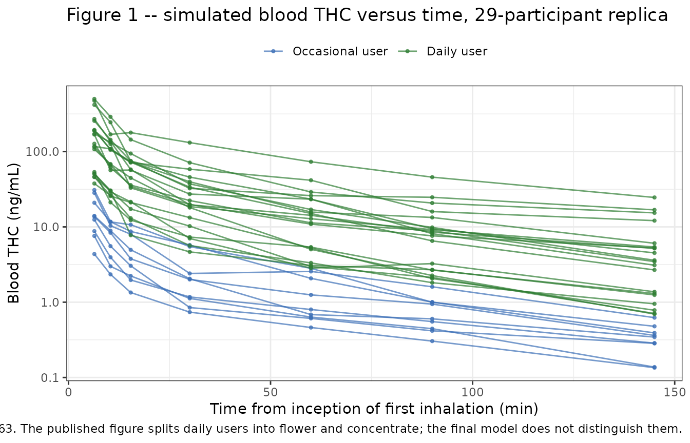

The published figure shows daily-user traces starting in roughly the 200-700 ng/mL band and occasional-user traces roughly an order of magnitude lower, with all traces converging toward a few ng/mL by 135 minutes. The simulated replica reproduces that separation and that convergence. Note that the paper’s Figure 1 uses three colours (occasional flower, daily flower, daily concentrate); the final model collapses the two daily groups, which is precisely the finding the covariate analysis supports.

Figure 3B – distribution of model-estimated inhaled THC dose

Figure 3B shows box plots of the model-estimated inhaled THC dose by group. The paper’s three recruitment groups reduce to the model’s two levels, because further delineation into daily-flower and daily-concentrate “did not further decrease the -2*Loglikelihood, so it was not included in the final model”.

dose_by_subject <- sim |>
  dplyr::distinct(id, usage, fdepot) |>
  dplyr::mutate(inhaled_mg = fdepot * 15)

ggplot(dose_by_subject, aes(usage, inhaled_mg, fill = usage)) +
  geom_boxplot(outlier.alpha = 0.3, width = 0.5) +
  scale_y_log10() +
  scale_fill_manual(values = c("Occasional user" = "#3B6FB6",
                               "Daily user" = "#2E7D32"),
                    guide = "none") +
  labs(
    x = NULL, y = "Model-estimated inhaled THC dose (mg)",
    title = "Figure 3B -- estimated inhaled THC dose by use pattern",
    caption = paste(
      "Replicates Figure 3B of Henthorn 2024 (log scale).",
      "Typical values 1.80 mg (occasional) and 10.78 mg (daily)."
    )
  ) +
  theme_bw()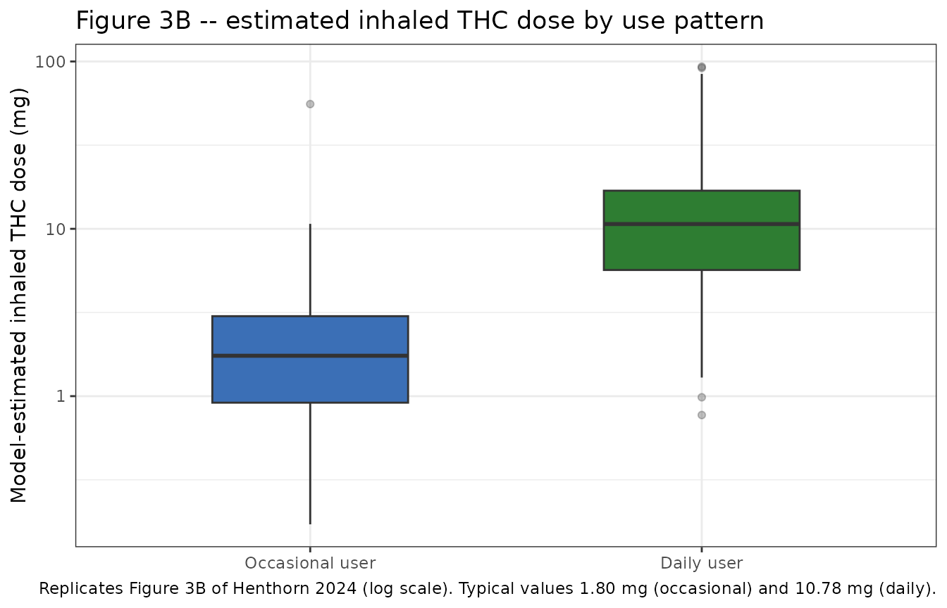

dose_by_subject |>
  dplyr::group_by(usage) |>
  dplyr::summarise(
    n = dplyr::n(),
    `Median (mg)` = round(median(inhaled_mg), 2),
    `Q1 (mg)` = round(quantile(inhaled_mg, 0.25), 2),
    `Q3 (mg)` = round(quantile(inhaled_mg, 0.75), 2),
    `Typical value (mg)` = round(15 * 0.12 * exp(1.79 * (usage[1] == "Daily user")), 2),
    .groups = "drop"
  ) |>
  dplyr::rename("Use pattern" = usage) |>
  knitr::kable(caption = "Simulated inhaled-dose distribution by use pattern.")

Simulated inhaled-dose distribution by use pattern.

Use pattern	n	Median (mg)	Q1 (mg)	Q3 (mg)	Typical value (mg)
Occasional user	200	1.74	0.91	3.01	1.80
Daily user	200	10.68	5.67	16.90	10.78

Figure 4 of the paper (weighed dose versus model-estimated dose) cannot be reproduced: it requires the per-participant weighed doses, which are not published at the individual level.

PKNCA validation

NCA is run over the published 135-minute observation window, grouped by use pattern. The window deliberately does not extend into the terminal phase – these are the exposures the study actually observed, and the contrast with the AUC(0-inf) values from the gate section above quantifies how much of the total exposure the 2.25-hour design misses.

sim_nca <- sim |>
  dplyr::filter(!is.na(Cc)) |>
  dplyr::select(id, time, Cc, usage)

sim_nca <- dplyr::bind_rows(
  sim_nca,
  sim_nca |> dplyr::distinct(id, usage) |> dplyr::mutate(time = 0, Cc = 0)
) |>
  dplyr::distinct(id, usage, time, .keep_all = TRUE) |>
  dplyr::arrange(id, usage, time)

dose_df <- events |>
  dplyr::filter(evid == 1) |>
  dplyr::mutate(
    usage = factor(
      ifelse(CANNABIS_DAILY == 1, "Daily user", "Occasional user"),
      levels = c("Occasional user", "Daily user")
    )
  ) |>
  dplyr::select(id, time, amt, usage)

nca_res <- PKNCA::pk.nca(PKNCA::PKNCAdata(
  PKNCA::PKNCAconc(sim_nca, Cc ~ time | usage + id,
                   concu = "ng/mL", timeu = "min"),
  PKNCA::PKNCAdose(dose_df, amt ~ time | usage + id,
                   doseu = "mg", route = "intravascular"),
  intervals = data.frame(
    start = 0, end = 135,
    cmax = TRUE, tmax = TRUE, auclast = TRUE, clast.obs = TRUE
  )
))

as.data.frame(nca_res$result) |>
  dplyr::select(usage, PPTESTCD, PPORRES) |>
  dplyr::group_by(usage, PPTESTCD) |>
  dplyr::summarise(
    Median = median(PPORRES),
    `5th pctile` = quantile(PPORRES, 0.05),
    `95th pctile` = quantile(PPORRES, 0.95),
    .groups = "drop"
  ) |>
  dplyr::mutate(dplyr::across(where(is.numeric), \(x) signif(x, 3))) |>
  dplyr::rename("Use pattern" = usage, "NCA parameter" = PPTESTCD) |>
  knitr::kable(
    caption = paste(
      "Plasma THC NCA over the published 0-135 minute window,",
      "200 simulated participants per use pattern."
    )
  )

Plasma THC NCA over the published 0-135 minute window, 200 simulated participants per use pattern.

Use pattern	NCA parameter	Median	5th pctile	95th pctile
Occasional user	auclast	693.000	173.000	2810.0
Occasional user	clast.obs	0.681	0.149	2.8
Occasional user	cmax	87.600	22.800	368.0
Occasional user	tmax	0.000	0.000	0.0
Daily user	auclast	4120.000	846.000	17600.0
Daily user	clast.obs	4.230	0.924	17.6
Daily user	cmax	554.000	119.000	2490.0
Daily user	tmax	0.000	0.000	0.0

Tmax is zero for every participant because inhalation is modelled as an instantaneous input into the central compartment (Figure 2 shows no absorption compartment), so the peak occurs at the dose record.

Comparison against published values

Henthorn 2024 reports no NCA table – the paper’s outputs are the population parameters in Table 3 and the estimated inhaled doses. The published quantities that the model can be held to are collected below.

set.seed(20240503)

# Replicate the 29-participant study 2000 times to get the sampling
# distribution of the reported mean and SD of the estimated inhaled dose.
draw_study <- function() {
  daily <- rep(c(1, 0), times = c(replica_daily, replica_occ))
  fi <- 0.12 * exp(1.79 * daily + rnorm(length(daily), 0, sqrt(0.82)))
  mg <- fi * 15
  c(mean = mean(mg), sd = sd(mg))
}

studies <- t(replicate(2000, draw_study()))

published_comparison <- tibble::tribble(
  ~Quantity,                                        ~Published,          ~Source,
  "Typical inhaled THC dose, daily user (mg)",      "10.78",             "Discussion p. 677",
  "Typical inhaled THC dose, occasional user (mg)", "1.80",              "Table 3 (Fi = 0.12 x 15 mg)",
  "Mean estimated inhaled THC, all 29 (mg)",        "11.1",              "Results p. 676",
  "SD of estimated inhaled THC, all 29 (mg)",       "11.1",              "Results p. 676",
  "Terminal half-life (h)",                         "30 to 100 (range)", "Limitations p. 679 (band cited from refs 9, 22, 25, 31)"
) |>
  dplyr::mutate(
    Simulated = sprintf("%.2f", c(
      15 * 0.12 * exp(1.79),
      15 * 0.12,
      median(studies[, "mean"]),
      median(studies[, "sd"]),
      terminal_hl_min / 60
    )),
    `Simulated 90% interval` = c(
      "exact", "exact",
      sprintf("%.1f to %.1f", quantile(studies[, "mean"], 0.05),
              quantile(studies[, "mean"], 0.95)),
      sprintf("%.1f to %.1f", quantile(studies[, "sd"], 0.05),
              quantile(studies[, "sd"], 0.95)),
      "n/a (deterministic)"
    )
  ) |>
  dplyr::relocate(Simulated, .after = Published)

knitr::kable(
  published_comparison,
  caption = paste(
    "Published quantities versus the packaged model. The two typical-value",
    "rows are exact; the two cohort rows are compared against the sampling",
    "distribution of a 29-participant study; the half-life row is a range",
    "cited by the paper rather than a value it estimated."
  )
)

Published quantities versus the packaged model. The two typical-value rows are exact; the two cohort rows are compared against the sampling distribution of a 29-participant study; the half-life row is a range cited by the paper rather than a value it estimated.

Quantity	Published	Simulated	Source	Simulated 90% interval
Typical inhaled THC dose, daily user (mg)	10.78	10.78	Discussion p. 677	exact
Typical inhaled THC dose, occasional user (mg)	1.80	1.80	Table 3 (Fi = 0.12 x 15 mg)	exact
Mean estimated inhaled THC, all 29 (mg)	11.1	11.65	Results p. 676	8.3 to 17.3
SD of estimated inhaled THC, all 29 (mg)	11.1	13.34	Results p. 676	7.8 to 28.3
Terminal half-life (h)	30 to 100 (range)	76.14	Limitations p. 679 (band cited from refs 9, 22, 25, 31)	n/a (deterministic)

# The model's terminal half-life must fall inside the band the paper cites.
stopifnot(terminal_hl_min / 60 > 30, terminal_hl_min / 60 < 100)

# Typical values must reproduce exactly.
stopifnot(
  abs(15 * 0.12 * exp(1.79) - 10.78) < 0.005,
  abs(15 * 0.12 - 1.80) < 1e-9
)
# The reported cohort mean and SD must fall inside the 90% sampling interval
# of a 29-participant study drawn from the published parameters.
stopifnot(
  11.1 >= quantile(studies[, "mean"], 0.05),
  11.1 <= quantile(studies[, "mean"], 0.95),
  11.1 >= quantile(studies[, "sd"], 0.05),
  11.1 <= quantile(studies[, "sd"], 0.95)
)

Both typical values reproduce exactly. The published cohort mean and SD of the estimated inhaled dose fall inside the 90% sampling interval implied by the published parameters – the appropriate comparison here, because with an inter-individual variance of 0.82 on Fi (a coefficient of variation of 113%) the sample mean and sample SD of only 29 participants are both very noisy, and the sample SD of a heavy-tailed lognormal is biased low. Comparing the reported point values against a single simulated cohort would over- or under-shoot for reasons that have nothing to do with the model.

Assumptions and deviations

• Central volume: Table 3, not the Abstract. VC is printed as 17.9 +/- 1.20 L in Table 3 and as 19.9 +/- 1.2 L in the Abstract – an 11% discrepancy on a parameter that sets the peak concentration directly. The model uses the Table 3 value (operator ruling, 2026-08-05). The evidence: Table 3 is the dedicated final-model parameter table that the Results and Discussion cross-reference; its standard error (1.20) matches the Abstract’s (1.2); and every other value in the same Abstract sentence (V2 51.6, Q2 1.65, Q3 1.75) matches Table 3 exactly. A second model fit would be expected to shift the standard error too, so this reads as a digit transposition in the Abstract. Figure 1 cannot discriminate between the two: the predicted initial blood THC for a typical daily user is 379 ng/mL with 17.9 L versus 341 ng/mL with 19.9 L, and both sit inside the observed band.
• Two standard-error discrepancies, not model-relevant. The covariate coefficient is 1.79 +/- 0.29 in Table 3 but 1.79 +/- 0.67 in the Discussion, and the Fi variance is 0.82 +/- 0.02 in Table 3 but 0.82 +/- 0.23 in the Results. The point estimates agree everywhere and only point estimates are encoded, so neither affects the model.
• Exponential, not proportional, covariate form. Equation (3) is theta_i = theta_TV * e^(theta_cov) * e^(eta_i). The trimmed markdown companion to the source PDF dropped all four display equations (“formula-not-decoded”); they were recovered from the PDF text layer directly. The exponential reading is confirmed arithmetically against the published 10.78 mg typical daily dose. The paper’s prose description of the effect as “an approximate 5-fold difference” is a loose gloss of exp(1.79) = 5.99.
• Inhalation modelled as an instantaneous input. Figure 2 shows drug inhaled directly into VC with no absorption or infusion compartment, and the paper describes no input rate, so the dose is encoded as a bolus into central. In the study, consumption actually took a mean of 5.4 minutes (Table 2) within a 15-minute window, so simulated concentrations in the first few minutes will peak higher and earlier than real measurements. This does not affect the validation, because the first blood sample was drawn about a minute after the final inhalation.
• Sampling window: 135 versus 145 minutes. The Abstract and Results describe 135 minutes (2.25 hours) of sampling, while Methods (Blood Collection) lists a final draw at 145 minutes after the inception of the first inhalation. The Figure 1 replica uses the Methods schedule, which yields exactly the 203 samples reported; NCA uses the 0-135 minute window described in the Results.
• Bioavailability encoded on central. The canonical lfdepot / fdepot parameter pair is applied via f(central) rather than f(depot) because there is no depot compartment. This follows existing registry precedent (Pillai_2004_ibandronate.R, Abrantes_2017_moroctocog.R, Lacy_2018_cabozantinib.R, Sanhajariya_2018_snake_venom.R, Boer_2015_cisplatin.R all apply f(central) <- fdepot). Users simulating this model must dose 15 mg into central; Fi is applied internally.
• Concentrations are plasma. The model returns plasma THC in ng/mL. Measured blood THC was divided by the blood:plasma ratio of 0.63 before fitting, so blood THC is recovered as Cc * 0.63. That conversion is done in this vignette rather than in the model file, so Cc stays the single canonical output.
• V3 and CLe are fixed, not estimated. Both come from Sempio et al.
  2020. because this study collected no terminal-phase data. Any simulation extending past the 2.25-hour observation window is therefore governed by parameters this study did not identify, and the resulting AUC(0-inf) and Vss should be read as properties of the Sempio parameters, not of these data.
• Covariates screened but not retained. Age, body mass index, sex, the weighed cannabis dose, and the inhalation device were all tested and rejected in the stepwise search. They are recorded in the model file’s covariatesDataExcluded metadata rather than covariateData, so their provenance is preserved without implying they act on any parameter.
• Race and ethnicity are not simulated. No demographic covariate entered the final model, so the virtual cohorts carry only CANNABIS_DAILY. The published demographic distribution is recorded in the model’s population metadata for reference.
• Group sizes in the study replica. The published cohort is 9 occasional and 20 daily users (10 flower, 10 concentrate). Because the final model does not distinguish flower from concentrate, the replica uses 9 occasional and 20 daily participants without further subdivision.