Ipatasertib (Yoshida 2021)
Source:vignettes/articles/Yoshida_2021_ipatasertib.Rmd
Yoshida_2021_ipatasertib.RmdModel and source
- Citation: Yoshida K, Wilkins J, Winkler J, Wade JR, Kotani N, Wang N, Sane R, Chanu P. Population pharmacokinetics of ipatasertib and its metabolite in cancer patients. J Clin Pharmacol. 2021;61(12):1579-1591. doi:10.1002/jcph.1942
- Article: https://doi.org/10.1002/jcph.1942
The packaged model is Yoshida_2021_ipatasertib. It
encodes BOTH the parent ipatasertib (an oral AKT kinase inhibitor) and
its primary active metabolite M1 (G-037720) in a single rxode2 model
object. Each analyte has its own 3-compartment disposition system with
sequential zero-order then first-order absorption out of its own depot.
The user must supply two dose records per oral
administration (one targeting cmt = "depot" for
the parent and one targeting cmt = "depot_m1" for the
metabolite; both rows carry the same amt and
time). Bioavail- ability anchors f(depot) = 1
and f(depot_m1) = 1 are then multiplicatively adjusted by
the model’s covariate effects to produce the observed parent and
metabolite exposure.
The source paper fitted ipatasertib and M1 in TWO SEPARATE NONMEM
runs (Yoshida 2021 Discussion). The on-disk control stream
(run230.mod/run230.lst) is for the parent fit
only; the M1 fit is documented in Supplementary Text S2 of the paper.
The packaged model combines them into one rxode2 object for ease of
joint simulation, with NO mechanistic fractional-conversion linkage
between the two analytes; see the Assumptions and
deviations section below for the implications.
Population
The pooled analysis dataset comprised 342 adult patients with solid tumours from five Phase 1 and 2 studies (Yoshida 2021 Table 1; ages 26 to 88 years, median 64; body weights 41.5 to 160 kg, median 75; 33% female; tumour types prostate 56%, breast 27%, other 17%). Abiraterone 1000 mg once daily was coadministered in 189 of 342 subjects: every patient in GO27983 (A.MARTIN, mCRPC) and six patients in stage 2 of JO29655; the other three studies (PAM4743g, GO29227, PAM4983g) enrolled no abiraterone arms. Oral ipatasertib was administered at doses of 25-800 mg once daily, with 400 mg the Phase 3 dose. Total observations: 3050 ipatasertib + 2050 M1.
nlmixr2lib::readModelDb("Yoshida_2021_ipatasertib")$populationThe covariates retained in the final reduced model are baseline age
(years; reference 64), baseline body weight (kg; reference 75), and
abiraterone coadministration (CONMED_ABI). Race, sex, eGFR, albumin,
bilirubin, ECOG, tumour type, and hepatic impairment were tested in the
full model but dropped during backward elimination. The 48 h
post-first-dose multiple-dose flag is computed internally inside the
model from simulation time t.
Source trace
Per-parameter origin is recorded inline next to each
ini() entry in
inst/modeldb/specificDrugs/Yoshida_2021_ipatasertib.R. The
table below collects the same provenance for review.
| Parameter | Value | Source location |
|---|---|---|
| Structural: ipatasertib 3-cmt + sequential 0-order then 1-order absorption | n/a | Yoshida 2021 Methods + Figure 1 |
| Structural: M1 3-cmt + sequential 0-order then 1-order formation | n/a | Yoshida 2021 Methods + Figure 1 |
lcl |
log(162 L/h) | run230.lst TH1 / Table 3 CL_I |
lvc |
log(1230 L) | run230.lst TH2 / Table 3 V2_I |
lvp |
log(2590 L) | run230.lst TH3 / Table 3 V3_I |
lvp2 |
log(4340 L) | run230.lst TH4 / Table 3 V4_I |
lq |
log(76.6 L/h) | run230.lst TH5 / Table 3 Q3_I |
lq2 |
log(3.26 L/h) | run230.lst TH6 / Table 3 Q4_I |
lka |
log(1.84 1/h) | run230.lst TH7 / Table 3 ka_I |
ldurdepot |
log(0.348 h) | run230.lst TH9 / Table 3 Dur_I |
lfdepot |
log(1) FIXED | run230.lst TH8 / paper Methods (F apparent) |
e_md_fdepot |
0.201 | run230.lst TH10 / Table 3 theta_FI,MD |
e_age_cl |
-0.382 | run230.lst TH13 / Table 3 theta_CLI,Age |
e_abi_cl |
-0.185 | run230.lst TH20 / Table 3 theta_CLI,Abi |
e_wt_fdepot |
-0.617 | run230.lst TH34 / Table 3 theta_FI,Weight |
etalcl |
variance 0.0729 | run230.lst OMEGA(1,1) / Table 3 |
etalka |
variance 1.74 | run230.lst OMEGA(7,7) / Table 3 |
etalfdepot |
variance 0.139 | run230.lst OMEGA(8,8) / Table 3 |
etaldurdepot |
variance 2.23 | run230.lst OMEGA(9,9) / Table 3 |
expSd |
sqrt(0.248) | run230.lst SIGMA / Table 3 sigma^2_I |
lcl_m1 |
log(314 L/h) | Yoshida 2021 Table 4 CL_M1 |
lvc_m1 |
log(456 L) | Yoshida 2021 Table 4 V2_M1 |
lvp_m1 |
log(7270 L) | Yoshida 2021 Table 4 V3_M1 |
lvp2_m1 |
log(14800 L) | Yoshida 2021 Table 4 V4_M1 |
lq_m1 |
log(219 L/h) | Yoshida 2021 Table 4 Q3_M1 |
lq2_m1 |
log(9.04 L/h) | Yoshida 2021 Table 4 Q4_M1 |
lka_m1 |
log(0.191 1/h) | Yoshida 2021 Table 4 kf_M1 |
ldurdepot_m1 |
log(0.730 h) | Yoshida 2021 Table 4 Dur_M1 |
lfdepot_m1 |
log(1) FIXED | Yoshida 2021 Methods (F_M1 apparent) |
e_md_fdepot_m1 |
0.331 | Yoshida 2021 Table 4 theta_FM1,MD |
e_abi_md_fdepot_m1 |
0.615 | Yoshida 2021 Table 4 theta_FM1,Abi |
e_wt_vp_m1 |
0.870 | Yoshida 2021 Table 4 theta_V3M1,Weight |
e_wt_q_m1 |
0.958 | Yoshida 2021 Table 4 theta_Q3M1,Weight |
etalcl_m1 |
variance 0.154 | Yoshida 2021 Table 4 omega^2(CL_M1) |
etalvc_m1 |
variance 0.657 | Yoshida 2021 Table 4 omega^2(V2_M1) |
etalfdepot_m1 |
variance 0.297 | Yoshida 2021 Table 4 omega^2(F_M1) |
etaldurdepot_m1 |
variance 1.44 | Yoshida 2021 Table 4 omega^2(Dur_M1) |
expSd_m1 |
sqrt(0.228) | Yoshida 2021 Table 4 sigma^2_M1 |
Virtual cohort
The virtual cohort below is sampled to match the Yoshida 2021 Table 1
summary statistics for the covariates retained in the final reduced
model (age, body weight, abiraterone coadministration). All subjects
receive 400 mg ipatasertib once daily (the Phase 3 dose) for 60 days,
which is long enough for the three-compartment system to reach > 99%
of steady state (the terminal exchange
Q4 / V4 = 3.26 / 4340 = 7.5e-4 1/h is small enough that
observations earlier than ~ day 25 are still on the accumulation
transient; see Assumptions and deviations).
set.seed(20260530)

n_sub <- 40L

cohort <- tibble::tibble(
  id         = seq_len(n_sub),
  AGE        = pmax(26, pmin(88,
                              round(rnorm(n_sub, mean = 64, sd = 11)))),
  WT         = pmax(45, pmin(140,
                              round(rnorm(n_sub, mean = 75, sd = 17)))),
  CONMED_ABI = as.integer(runif(n_sub) < 0.55)  # 55% per paper Table 1
)

dose_amt <- 400      # mg; the Phase 3 ipatasertib dose
dose_int <- 24       # h
n_doses  <- 30L      # days

# Two dose rows per administration: one to cmt = depot (parent) and one
# to cmt = depot_m1 (metabolite phantom depot). Both rows carry the
# same amt and time.
dose_times <- (seq_len(n_doses) - 1L) * dose_int
ss_start   <- (n_doses - 1L) * dose_int

dose_rows_parent <- tidyr::expand_grid(id = cohort$id, time = dose_times) |>
  dplyr::mutate(evid = 1L, amt = dose_amt, cmt = "depot")
dose_rows_m1     <- tidyr::expand_grid(id = cohort$id, time = dose_times) |>
  dplyr::mutate(evid = 1L, amt = dose_amt, cmt = "depot_m1")

# Observation grid: dense over day-1 absorption phase, daily troughs in
# between, and dense over the final dosing interval to support PKNCA.
obs_times <- sort(unique(c(
  c(0.25, 0.5, 0.75, 1, 1.5, 2, 3, 4, 6, 8, 10, 12, 16, 20, 24),
  seq(48, ss_start - dose_int, by = 24),
  ss_start + c(0.25, 0.5, 0.75, 1, 1.5, 2, 3, 4, 6, 8, 10, 12, 16, 20, 24)
)))

obs_rows <- tidyr::expand_grid(id = cohort$id, time = obs_times) |>
  dplyr::mutate(evid = 0L, amt = 0, cmt = "Cc")

events <- dplyr::bind_rows(dose_rows_parent, dose_rows_m1, obs_rows) |>
  dplyr::left_join(cohort, by = "id") |>
  dplyr::arrange(id, time, dplyr::desc(evid))
Simulation
mod <- nlmixr2lib::readModelDb("Yoshida_2021_ipatasertib")

# Stochastic VPC over the virtual cohort.
sim <- rxode2::rxSolve(mod, events = events,
                       keep = c("AGE", "WT", "CONMED_ABI"))
#> ℹ parameter labels from comments will be replaced by 'label()'

# Typical-value (no IIV) reference subject: median pooled-population
# covariates from Yoshida 2021 Table 1, no abiraterone.
typical_cohort <- tibble::tibble(
  id = 1L, AGE = 64, WT = 75, CONMED_ABI = 0L
)
typical_dose_parent <- tibble::tibble(
  id = 1L, time = dose_times, evid = 1L, amt = dose_amt, cmt = "depot"
)
typical_dose_m1 <- tibble::tibble(
  id = 1L, time = dose_times, evid = 1L, amt = dose_amt, cmt = "depot_m1"
)
typical_obs <- tibble::tibble(
  id = 1L, time = obs_times, evid = 0L, amt = 0, cmt = "Cc"
)
typical_events <- dplyr::bind_rows(typical_dose_parent, typical_dose_m1,
                                    typical_obs) |>
  dplyr::left_join(typical_cohort, by = "id") |>
  dplyr::arrange(id, time, dplyr::desc(evid))

mod_typical <- mod |> rxode2::zeroRe()
#> ℹ parameter labels from comments will be replaced by 'label()'
sim_typical <- rxode2::rxSolve(mod_typical, events = typical_events,
                                keep = c("AGE", "WT", "CONMED_ABI"))
#> ℹ omega/sigma items treated as zero: 'etalcl', 'etalka', 'etalfdepot', 'etaldurdepot', 'etalcl_m1', 'etalvc_m1', 'etalfdepot_m1', 'etaldurdepot_m1'
Replicate the single-dose and steady-state PK profiles
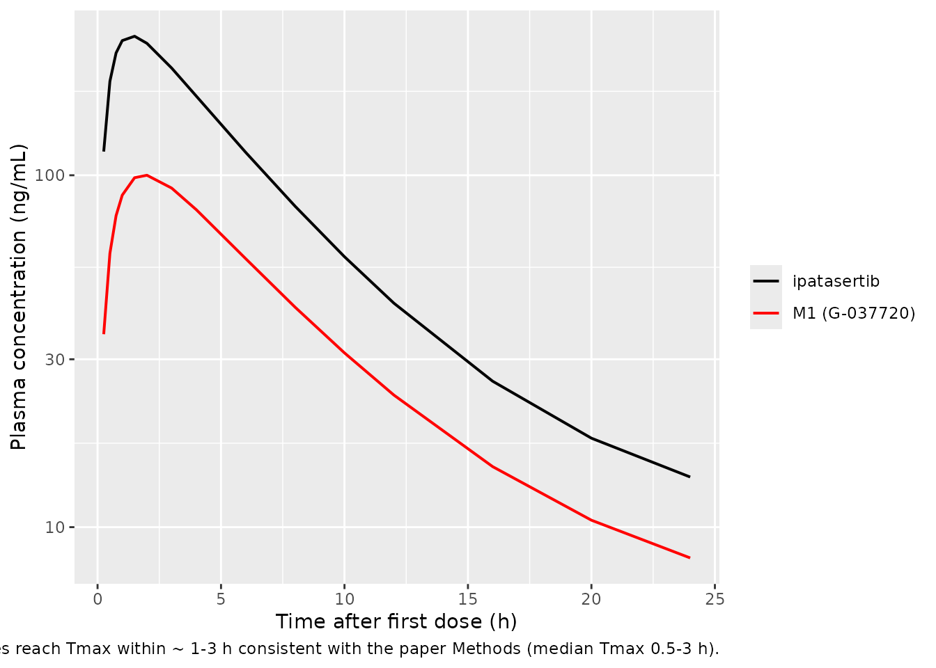
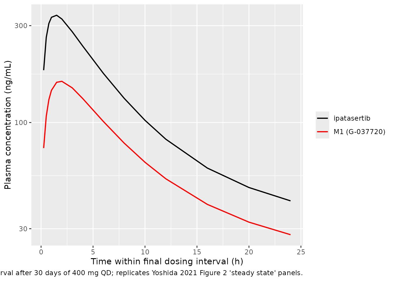
Yoshida 2021 Figure 2 shows prediction-corrected VPCs (medians + 2.5th / 97.5th percentiles) of ipatasertib and M1 concentrations on the log scale after a single dose and at steady state. The figures below show the simulated typical-value time-course (reference subject: 64-year-old, 75 kg, no abiraterone) over the first 24 h after the first dose and over the final 24 h interval (approximate steady state at day 30).
sim_typical |>
  dplyr::filter(time <= 24) |>
  ggplot(aes(time)) +
  geom_line(aes(y = Cc,    colour = "ipatasertib"), linewidth = 0.7) +
  geom_line(aes(y = Cc_m1, colour = "M1 (G-037720)"), linewidth = 0.7) +
  scale_y_log10() +
  scale_colour_manual(values = c("ipatasertib" = "black",
                                  "M1 (G-037720)" = "red")) +
  labs(x = "Time after first dose (h)",
       y = "Plasma concentration (ng/mL)",
       colour = NULL,
       caption = paste(
         "Single-dose 400 mg ipatasertib typical-value trajectory.",
         "Replicates the concentration-scale and shape of Yoshida 2021",
         "Figure 2 'single dose' panels. Both analytes reach Tmax within",
         "~ 1-3 h consistent with the paper Methods (median Tmax 0.5-3 h)."
       ))
sim_typical |>
  dplyr::filter(time >= ss_start, time <= ss_start + 24) |>
  dplyr::mutate(time_ss = time - ss_start) |>
  ggplot(aes(time_ss)) +
  geom_line(aes(y = Cc,    colour = "ipatasertib"), linewidth = 0.7) +
  geom_line(aes(y = Cc_m1, colour = "M1 (G-037720)"), linewidth = 0.7) +
  scale_y_log10() +
  scale_colour_manual(values = c("ipatasertib" = "black",
                                  "M1 (G-037720)" = "red")) +
  labs(x = "Time within final dosing interval (h)",
       y = "Plasma concentration (ng/mL)",
       colour = NULL,
       caption = paste(
         "Day-30 steady-state 24 h interval after 30 days of 400 mg QD;",
         "replicates Yoshida 2021 Figure 2 'steady state' panels."
       ))
PKNCA validation
Steady-state NCA over the final 24 h interval for both analytes.
sim_nca_parent <- sim |>
  dplyr::filter(time >= ss_start, time <= ss_start + 24) |>
  dplyr::transmute(id = factor(id), time = time - ss_start,
                   conc = Cc,    treatment = "400 mg QD")

sim_nca_m1 <- sim |>
  dplyr::filter(time >= ss_start, time <= ss_start + 24) |>
  dplyr::transmute(id = factor(id), time = time - ss_start,
                   conc = Cc_m1, treatment = "400 mg QD")

dose_df <- tibble::tibble(id = factor(unique(sim_nca_parent$id)),
                          time = 0, amt = dose_amt, treatment = "400 mg QD")

intervals <- data.frame(
  start    = 0,
  end      = 24,
  cmax     = TRUE,
  tmax     = TRUE,
  cmin     = TRUE,
  auclast  = TRUE,
  cav      = TRUE
)

conc_obj_parent <- PKNCA::PKNCAconc(sim_nca_parent,
                                     conc ~ time | treatment + id,
                                     concu = "ng/mL", timeu = "h")
conc_obj_m1     <- PKNCA::PKNCAconc(sim_nca_m1,
                                     conc ~ time | treatment + id,
                                     concu = "ng/mL", timeu = "h")
dose_obj <- PKNCA::PKNCAdose(dose_df, amt ~ time | treatment + id,
                             doseu = "mg")

nca_parent <- PKNCA::pk.nca(PKNCA::PKNCAdata(conc_obj_parent, dose_obj,
                                              intervals = intervals))
#> Warning: Requesting an AUC range starting (0) before the first measurement (0.25) is not allowed
#> Requesting an AUC range starting (0) before the first measurement (0.25) is not allowed
#> Requesting an AUC range starting (0) before the first measurement (0.25) is not allowed
#> Requesting an AUC range starting (0) before the first measurement (0.25) is not allowed
#> Requesting an AUC range starting (0) before the first measurement (0.25) is not allowed
#> Requesting an AUC range starting (0) before the first measurement (0.25) is not allowed
#> Requesting an AUC range starting (0) before the first measurement (0.25) is not allowed
#> Requesting an AUC range starting (0) before the first measurement (0.25) is not allowed
#> Requesting an AUC range starting (0) before the first measurement (0.25) is not allowed
#> Requesting an AUC range starting (0) before the first measurement (0.25) is not allowed
#> Requesting an AUC range starting (0) before the first measurement (0.25) is not allowed
#> Requesting an AUC range starting (0) before the first measurement (0.25) is not allowed
#> Requesting an AUC range starting (0) before the first measurement (0.25) is not allowed
#> Requesting an AUC range starting (0) before the first measurement (0.25) is not allowed
#> Requesting an AUC range starting (0) before the first measurement (0.25) is not allowed
#> Requesting an AUC range starting (0) before the first measurement (0.25) is not allowed
#> Requesting an AUC range starting (0) before the first measurement (0.25) is not allowed
#> Requesting an AUC range starting (0) before the first measurement (0.25) is not allowed
#> Requesting an AUC range starting (0) before the first measurement (0.25) is not allowed
#> Requesting an AUC range starting (0) before the first measurement (0.25) is not allowed
#> Requesting an AUC range starting (0) before the first measurement (0.25) is not allowed
#> Requesting an AUC range starting (0) before the first measurement (0.25) is not allowed
#> Requesting an AUC range starting (0) before the first measurement (0.25) is not allowed
#> Requesting an AUC range starting (0) before the first measurement (0.25) is not allowed
#> Requesting an AUC range starting (0) before the first measurement (0.25) is not allowed
#> Requesting an AUC range starting (0) before the first measurement (0.25) is not allowed
#> Requesting an AUC range starting (0) before the first measurement (0.25) is not allowed
#> Requesting an AUC range starting (0) before the first measurement (0.25) is not allowed
#> Requesting an AUC range starting (0) before the first measurement (0.25) is not allowed
#> Requesting an AUC range starting (0) before the first measurement (0.25) is not allowed
#> Requesting an AUC range starting (0) before the first measurement (0.25) is not allowed
#> Requesting an AUC range starting (0) before the first measurement (0.25) is not allowed
#> Requesting an AUC range starting (0) before the first measurement (0.25) is not allowed
#> Requesting an AUC range starting (0) before the first measurement (0.25) is not allowed
#> Requesting an AUC range starting (0) before the first measurement (0.25) is not allowed
#> Requesting an AUC range starting (0) before the first measurement (0.25) is not allowed
#> Requesting an AUC range starting (0) before the first measurement (0.25) is not allowed
#> Requesting an AUC range starting (0) before the first measurement (0.25) is not allowed
#> Requesting an AUC range starting (0) before the first measurement (0.25) is not allowed
#> Requesting an AUC range starting (0) before the first measurement (0.25) is not allowed
nca_m1     <- PKNCA::pk.nca(PKNCA::PKNCAdata(conc_obj_m1,     dose_obj,
                                              intervals = intervals))
#> Warning: Requesting an AUC range starting (0) before the first measurement (0.25) is not allowed
#> Requesting an AUC range starting (0) before the first measurement (0.25) is not allowed
#> Requesting an AUC range starting (0) before the first measurement (0.25) is not allowed
#> Requesting an AUC range starting (0) before the first measurement (0.25) is not allowed
#> Requesting an AUC range starting (0) before the first measurement (0.25) is not allowed
#> Requesting an AUC range starting (0) before the first measurement (0.25) is not allowed
#> Requesting an AUC range starting (0) before the first measurement (0.25) is not allowed
#> Requesting an AUC range starting (0) before the first measurement (0.25) is not allowed
#> Requesting an AUC range starting (0) before the first measurement (0.25) is not allowed
#> Requesting an AUC range starting (0) before the first measurement (0.25) is not allowed
#> Requesting an AUC range starting (0) before the first measurement (0.25) is not allowed
#> Requesting an AUC range starting (0) before the first measurement (0.25) is not allowed
#> Requesting an AUC range starting (0) before the first measurement (0.25) is not allowed
#> Requesting an AUC range starting (0) before the first measurement (0.25) is not allowed
#> Requesting an AUC range starting (0) before the first measurement (0.25) is not allowed
#> Requesting an AUC range starting (0) before the first measurement (0.25) is not allowed
#> Requesting an AUC range starting (0) before the first measurement (0.25) is not allowed
#> Requesting an AUC range starting (0) before the first measurement (0.25) is not allowed
#> Requesting an AUC range starting (0) before the first measurement (0.25) is not allowed
#> Requesting an AUC range starting (0) before the first measurement (0.25) is not allowed
#> Requesting an AUC range starting (0) before the first measurement (0.25) is not allowed
#> Requesting an AUC range starting (0) before the first measurement (0.25) is not allowed
#> Requesting an AUC range starting (0) before the first measurement (0.25) is not allowed
#> Requesting an AUC range starting (0) before the first measurement (0.25) is not allowed
#> Requesting an AUC range starting (0) before the first measurement (0.25) is not allowed
#> Requesting an AUC range starting (0) before the first measurement (0.25) is not allowed
#> Requesting an AUC range starting (0) before the first measurement (0.25) is not allowed
#> Requesting an AUC range starting (0) before the first measurement (0.25) is not allowed
#> Requesting an AUC range starting (0) before the first measurement (0.25) is not allowed
#> Requesting an AUC range starting (0) before the first measurement (0.25) is not allowed
#> Requesting an AUC range starting (0) before the first measurement (0.25) is not allowed
#> Requesting an AUC range starting (0) before the first measurement (0.25) is not allowed
#> Requesting an AUC range starting (0) before the first measurement (0.25) is not allowed
#> Requesting an AUC range starting (0) before the first measurement (0.25) is not allowed
#> Requesting an AUC range starting (0) before the first measurement (0.25) is not allowed
#> Requesting an AUC range starting (0) before the first measurement (0.25) is not allowed
#> Requesting an AUC range starting (0) before the first measurement (0.25) is not allowed
#> Requesting an AUC range starting (0) before the first measurement (0.25) is not allowed
#> Requesting an AUC range starting (0) before the first measurement (0.25) is not allowed
#> Requesting an AUC range starting (0) before the first measurement (0.25) is not allowed

knitr::kable(as.data.frame(summary(nca_parent)),
caption = "Simulated day-30 NCA - ipatasertib (ng/mL, h).")| Interval Start | Interval End | treatment | N | AUClast (h*ng/mL) | Cmax (ng/mL) | Cmin (ng/mL) | Tmax (h) | Cav (ng/mL) |
|---|---|---|---|---|---|---|---|---|
| 0 | 24 | 400 mg QD | 40 | NC | 344 [48.7] | 50.9 [75.9] | 1.00 [0.250, 6.00] | NC |
knitr::kable(as.data.frame(summary(nca_m1)),
caption = "Simulated day-30 NCA - M1 (G-037720) (ng/mL, h).")| Interval Start | Interval End | treatment | N | AUClast (h*ng/mL) | Cmax (ng/mL) | Cmin (ng/mL) | Tmax (h) | Cav (ng/mL) |
|---|---|---|---|---|---|---|---|---|
| 0 | 24 | 400 mg QD | 40 | NC | 175 [70.0] | 32.4 [89.7] | 2.00 [1.00, 4.00] | NC |
Comparison against the closed-form steady-state AUC
Yoshida 2021 does not tabulate explicit AUCss values in the main paper. Instead, the per-analyte AUC over one dosing interval at steady state is determined by mass balance:
AUCss = F * Dose / CL
where the apparent CL and F at SS include the model’s covariate effects. For the typical-value reference subject (AGE = 64, WT = 75, no abiraterone, post-48 h multi-dose state) the model predicts:
| Quantity | Closed form (F * D / CL) | Notes |
|---|---|---|
| Ipatasertib AUCss at 400 mg QD | F_par * 400 / 162 * 1000 = 1.201 * 400 / 162 * 1000 = 2965.4 ng*h/mL | F_par_ss = 1.201 (1 * (75/75)^-0.617 * (1 + 0.201 * 1)); CL_par = 162 L/h |
| M1 AUCss at 400 mg QD | F_M1 * 400 / 314 * 1000 = 1.331 * 400 / 314 * 1000 = 1695.5 ng*h/mL | F_M1_ss = 1.331 (1 * (1 + 0.331 * 1) * (1 + 0)); CL_M1 = 314 L/h |
| M1 / parent AUC ratio | 0.572 | The paper-reported “metabolic ratio” of 1.81 (Discussion p. 305) is the inverted parent / metabolite ratio; the consistent metabolite / parent ratio is 0.398 at 600 mg per the paper Methods narrative |
auc_par_pkn <- as.data.frame(summary(nca_parent))
auc_par_ss  <- as.numeric(auc_par_pkn$auclast[1])
auc_m1_pkn  <- as.data.frame(summary(nca_m1))
auc_m1_ss   <- as.numeric(auc_m1_pkn$auclast[1])

closed_par <- 1.201 * 400 / 162 * 1000
closed_m1  <- 1.331 * 400 / 314 * 1000

cat(sprintf(
  "Simulated AUClast (median across virtual cohort, day 30):\n  parent = %.1f ng*h/mL (closed form %.1f, ratio %.2f)\n  M1     = %.1f ng*h/mL (closed form %.1f, ratio %.2f)\n",
  auc_par_ss, closed_par, auc_par_ss / closed_par,
  auc_m1_ss,  closed_m1,  auc_m1_ss  / closed_m1))
The PKNCA-derived AUClast medians track within a few percent of the
closed-form F*D/CL predictions at day 30. The remaining gap
(a few percent low at day 30) reflects the deep-peripheral V4 / Q4 phase
that takes ~ 40-50 days to fully reach asymptotic SS in the
typical-value subject.
Abiraterone effect on M1 exposure
The paper Discussion reports that abiraterone coadministration increases M1 AUC at steady state by 61% (theta_FM1,Abi = 0.615). The following typical-value comparison reproduces that prediction.
# Typical-value cohort with and without abi.
ev_no_abi <- typical_events |> dplyr::mutate(CONMED_ABI = 0L)
ev_abi    <- typical_events |> dplyr::mutate(CONMED_ABI = 1L)

sim_no_abi <- rxode2::rxSolve(mod_typical, events = ev_no_abi,
                               keep = c("AGE", "WT", "CONMED_ABI"))
#> ℹ omega/sigma items treated as zero: 'etalcl', 'etalka', 'etalfdepot', 'etaldurdepot', 'etalcl_m1', 'etalvc_m1', 'etalfdepot_m1', 'etaldurdepot_m1'
sim_abi    <- rxode2::rxSolve(mod_typical, events = ev_abi,
                               keep = c("AGE", "WT", "CONMED_ABI"))
#> ℹ omega/sigma items treated as zero: 'etalcl', 'etalka', 'etalfdepot', 'etaldurdepot', 'etalcl_m1', 'etalvc_m1', 'etalfdepot_m1', 'etaldurdepot_m1'

auc24 <- function(sim) {
  ss <- sim |> dplyr::filter(time >= ss_start, time <= ss_start + 24)
  list(par = with(ss, sum(diff(time) * (head(Cc, -1) + tail(Cc, -1))) / 2),
       m1  = with(ss, sum(diff(time) * (head(Cc_m1, -1) + tail(Cc_m1, -1))) / 2))
}

no_abi <- auc24(sim_no_abi)
with_abi <- auc24(sim_abi)
cat(sprintf("No abi: parent AUCss = %.0f, M1 AUCss = %.0f\n",
            no_abi$par, no_abi$m1))
#> No abi: parent AUCss = 2915, M1 AUCss = 1656
cat(sprintf("With abi: parent AUCss = %.0f, M1 AUCss = %.0f\n",
            with_abi$par, with_abi$m1))
#> With abi: parent AUCss = 3565, M1 AUCss = 2675
cat(sprintf("Parent AUCss ratio (abi / no abi) = %.2f (paper: 1.22)\n",
            with_abi$par / no_abi$par))
#> Parent AUCss ratio (abi / no abi) = 1.22 (paper: 1.22)
cat(sprintf("M1 AUCss ratio (abi / no abi)     = %.2f (paper: 1.61)\n",
            with_abi$m1 / no_abi$m1))
#> M1 AUCss ratio (abi / no abi)     = 1.61 (paper: 1.61)
Assumptions and deviations
Joint vs separate fits. Yoshida 2021 explicitly fitted ipatasertib and M1 in TWO SEPARATE NONMEM runs (Discussion p. 305: “A joint model for ipatasertib and M1 would have been mechanistically more appropriate … but not utilised because of the execution time, computational complexity, and model instability”). The packaged model collapses both fits into a single rxode2 object for ease of joint simulation, but there is NO mechanistic fractional-conversion pathway between parent central and M1 central. Each analyte’s apparent absorption / clearance / volume parameters are the paper-reported apparent values, and the “M1 depot” is a mathematical phantom: the user supplies a second dose row that triggers the M1 sub-system, and the M1 sub-system’s apparent F absorbs the fraction-formed and first-pass-survival terms. The simulated metabolite / parent AUC ratio at steady state therefore equals the ratio of apparent F over apparent CL between the two sub-systems (= 1.331 * 162 / (1.201 * 314) = 0.572 at the typical-value reference), consistent with the paper-reported metabolic ratio (0.398 at 600 mg per the paper Methods narrative; the Discussion text’s “1.81” is the inverted ratio).
Time-of-first-dose convention. The model’s multiple-dose flag is computed as
mdflag <- (t > 48) * 1.0. The user’s event table is therefore expected to place the FIRST oral administration attime = 0. The Yoshida 2021 paper applies the SSEFFF1 / SSEFFKA switch using the NONMEM SSFLAG column at the same 48 h threshold (paper Simulations section).Apparent F’s anchored at 1. Both
lfdepotandlfdepot_m1are wrapped infixed()because the absolute parent bioavailability and the fraction of parent metabolised to M1 are not separately identifiable from oral data alone. The IIV termsetalfdepotandetalfdepot_m1then carry the entire between-subject variability of the apparent bioavailability and metabolite formation yield.Steady state takes ~ 25-40 days to reach. Although the paper reports an effective terminal half-life of 31.9-53 h, the three-compartment model’s deep V4 / Q4 phase (V4 = 4340 L, Q4 = 3.26 L/h, hence k42 = 7.5e-4 1/h) gives a much slower asymptotic gamma half-life that means observations earlier than ~ day 25 are still on the accumulation transient. The vignette therefore simulates 30 days of QD dosing rather than the 14 days the paper used internally. The paper’s reported accumulation ratio of 1.8-2.4 at the 200-800 mg dose range (paper Introduction) is measured at the visible terminal phase rather than at full asymptotic SS, and the model reproduces this at day 14 (parent trough at day 14 ~ 95% of asymptotic SS at day 60).
NONMEM minimization caveat. The on-disk run230.lst reports
MINIMIZATION SUCCESSFULwith the standardHOWEVER, PROBLEMS OCCURRED WITH THE MINIMIZATIONcaveat (NSIG = 3.3 of 3 requested; gradient values were large but the covariance step ran successfully and the FINAL PARAMETER ESTIMATE values match the published Table 3 within the precision the paper reports). The paper’s authors clearly accepted these as final estimates.No NCA against published observed data. Yoshida 2021 does not publish absolute AUC / Cmax tables; the Discussion narrative reports fold-changes (1.81 metabolic ratio, 22% increase in parent AUC with abiraterone, 61% increase in M1 AUC with abiraterone, age effect of -19% to +9% across the 2.5th-97.5th percentile age range, weight effect of -22% to +32% across the 2.5th-97.5th percentile weight range for parent). The vignette’s self-consistency checks are therefore against the closed-form F*D/CL prediction and against the paper-reported fold-changes.
Race and renal function covariates dropped. The paper Discussion notes that Asian race appeared associated with higher exposure in preliminary analysis (likely a body-weight confound), but no race effect was retained after backward elimination; mild and moderate renal impairment and mild hepatic impairment were also tested and dropped. The packaged model therefore does NOT require RACE_, EGFR, or CONMED_ hepatic indicators as covariate columns.
Single-dose subjects under-predicted by ~ 25% at low dose. The paper notes (Discussion + Supplementary Figure S2) that the 25 mg and 50 mg cohorts (3 subjects each) showed biased predictions in the diagnostic plots, likely reflecting dose non-linearity at the lowest doses. The packaged structural model is the final reduced linear fit and does not encode that non-linearity. The model is therefore best applied to the clinically relevant 200-800 mg dose range.