Model and source
- Citation: Rini BI, Garrett M, Poland B, Dutcher JP, Rixe O, Wilding G, Stadler WM, Pithavala YK, Kim S, Tarazi J, Motzer RJ. Axitinib in metastatic renal cell carcinoma: results of a pharmacokinetic and pharmacodynamic analysis. J Clin Pharmacol. 2013;53(5):491-504. doi:10.1002/jcph.73
- Description: Two-compartment population PK model for axitinib pooled across healthy volunteers and patients with metastatic renal cell carcinoma or other solid tumours (Rini 2013). First-order absorption with an estimated lag time; linear-proportional effects of age > 60 years, Japanese ethnicity and active smoking on systemic clearance; power-form effect of body weight on the central volume of distribution (reference 74.1 kg); a linear-proportional fasting effect on the absorption rate constant ka; a linear-proportional fasting effect on bioavailability F that applies only to crystal polymorph Form IV; and a linear-proportional reduction in F for the marketed crystal polymorph Form XLI relative to Form IV. Pooled data from 590 subjects (383 healthy volunteers, 181 metastatic RCC patients and 26 patients with other solid tumours) across 17 trials.
- Article: https://doi.org/10.1002/jcph.73
Rini 2013 pooled plasma axitinib concentrations from 590 subjects
across 17 trials – 383 healthy volunteers, 181 patients with metastatic
renal cell carcinoma (mRCC), and 26 patients with other solid tumours
(Table 1) – and fit a single linear two-compartment population PK model
with first-order absorption and an estimated absorption lag time. Twelve
covariates were screened. Age > 60 years, Japanese ethnicity and
active smoking were retained on systemic clearance CL; body
weight was retained as a power function on the central volume
Vc. The food and crystal-polymorph effects of clinical
interest – fasting on the absorption rate constant ka and
on absolute oral bioavailability F, and the F
reduction for the marketed Form XLI polymorph relative to the earlier
Form IV – were carried in the model throughout.
Rini 2013 is the pooled healthy-volunteer-plus-patient analysis. This
library also ships Garrett_2014_axitinib, the companion
healthy-volunteer-only analysis by an overlapping author group; the two
models share a structure but not their parameter values or their
covariate sets, and neither supersedes the other.
The paper’s second half is an exposure-response analysis in a
168-patient mRCC subset: multivariate Cox proportional-hazards
regression for progression-free and overall survival, and logistic
regression for RECIST partial response. Those are not encoded in the
model file – see the Errata section for why – but the exposure metric
they are built on, AUC = total daily dose * F / CL, is
fully specified and is used as a validation target below.
Population
The pooled PK dataset (Rini 2013 Results “Subject characteristics”;
reproduced programmatically via
readModelDb("Rini_2013_axitinib")$population) covers 590
subjects with median (range) body weight 74 kg (37-136), creatinine
clearance 103 mL/min (8-214), AST 22 U/L (9-154), ALT 21 U/L (5-188) and
bilirubin 0.7 mg/dL (0.1-3). Overall median age is 42 years (18-85), but
the two sub-populations differ sharply: patients have a median age of 60
years (32-85) and healthy volunteers 32 years (18-69). Most subjects are
male (85%) and Caucasian (61%). Only 19 of 590 subjects (3%) were active
smokers. Normal renal and hepatic function were study-entry
requirements, which is why creatinine clearance, AST, ALT and bilirubin
all screened out.
Healthy volunteers received a single 5 mg oral dose (one study additionally gave 1 mg intravenously to anchor absolute bioavailability, and one Chinese study gave single 5, 7 and 10 mg doses); patients received 5 mg orally twice daily with titration up to 10 mg twice daily permitted. Sixteen hepatically impaired subjects (study 13) and sixteen study-1 patients started above the 5 mg bid maximum tolerated dose were excluded from the analysis dataset.
The exposure-response subset is 168 of the 178 patients enrolled in the three mRCC studies (Table 3): median age 60 years (34-85), 71% male, 68% cytokine-refractory and 32% sorafenib-refractory, 65% with baseline ECOG PS 0, median haemoglobin 12.4 g/dL and median corrected serum calcium 9.4 mg/dL.
Source trace
The per-parameter origin is recorded as an in-file comment next to
each ini() entry in
inst/modeldb/specificDrugs/Rini_2013_axitinib.R. The table
below collects them in one place for review.
| Equation / parameter | Value | Source location |
|---|---|---|
| Structural model – linear two-compartment, first-order absorption, absorption lag time | n/a | Methods “Model development”; Results “PK model” |
Reference body weight for the Vc power function |
74.1 kg | Results “PK model” typical-value equation (screening median body weight 74 kg) |
lka (fed reference) |
log(0.482) | Table 2 “k a (hour-1): fed” = 0.482 |
lcl |
log(14.6) | Table 2 “CL (L/h)” = 14.6 |
lvc (at 74.1 kg) |
log(47.3) | Table 2 “V c (L)” = 47.3 |
lq |
log(4.00) | Table 2 “Q (L/h)” = 4.00 |
lvp |
log(393) | Table 2 “V p (L)” = 393 |
lfdepot (Form IV, fed reference) |
log(0.457) | Table 2 “F: fed/Form IV” = 0.457 |
ltlag |
log(0.454) | Table 2 “t lag (hour)” = 0.454 |
e_age_cl (age > 60 y on CL) |
-0.213 | Table 2 “Age >60-yr effect on CL”; Results “PK model” equation
CL = 14.6 * (1 - 0.213 * Age>60) * ...
|
e_jpn_cl (Japanese on CL) |
-0.249 | Table 2 “Japanese ethnicity effect on CL”; Results “PK model”
equation ... * (1 - 0.249 * RaceJapanese) * ...
|
e_smoke_cl (active smoking on CL) |
1.02 | Table 2 “Smoking status on CL”; Results “PK model” equation
... * (1 + 1.02 * Smokeractive)
|
e_wt_vc (power exponent of WT on Vc) |
0.778 | Table 2 “Weight effect on V c”; Results “PK model” equation
Vc = 47.3 * (weight / 74.1 kg)^0.778
|
e_fast_ka (fasting on ka) |
1.97 | Table 2 “Fasting effect on k a”; footnote e:
ka_fasted = 0.482 * (1 + 1.97) = 1.43 /h
|
e_fast_f (fasting on F, Form IV only) |
0.330 | Table 2 “Fasting on F, Form IV”; footnote f:
F = 0.457 * (1 + 0.33) = 0.608
|
e_xli_f (Form XLI on F) |
-0.121 | Table 2 “Form XLI on F”; footnote g:
F = 0.457 * (1 - 0.121) = 0.402, and no food effect with
Form XLI |
omega^2 CL |
0.599^2 = 0.358801 | Table 2 “CL (L/h) 14.6 (59.9)” with footnote a (IIV given as %CV) |
omega^2 Vc |
0.397^2 = 0.157609 | Table 2 “V c (L) 47.3 (39.7)” |
omega^2 shared by Q and Vp |
0.868^2 = 0.753424 | Table 2 “Q (L/h) 4.00 (86.8)” with footnote d (Q and Vp 100% correlated, same IIV) |
omega^2 ka |
0.77^2 = 0.5929 | Table 2 “k a (hour-1): fed 0.482 (77)” |
expSd (oral log-scale residual SD) |
0.582 | Table 2 “Residual error (%), oral” = 58.2 |
| IV log-scale residual SD (not encoded) | 0.335 | Table 2 “Residual error (%), intravenous” = 33.5 (see Errata) |
| Exposure metric for the PK/PD analysis | AUC = total daily dose * F / CL |
Methods “PK/PD Modeling” |
| Published median mean-daily AUC, 168 mRCC patients | 375 h*ng/mL (32.8-1,728) | Table 3 “AUC, hxng/mL” |
| Cox regression coefficients for AUC and dBP | see Errata | Table 5 |
Typical-value covariate identities
Every covariate effect in Rini 2013 has a closed-form typical value that the paper either prints as an equation (Results “PK model”) or works out in a Table 2 footnote. Because both sides of these checks use the same parameters, the comparison is exact arithmetic and is asserted tightly.
mod     <- readModelDb("Rini_2013_axitinib")
mod_typ <- rxode2::zeroRe(mod)

# One subject per covariate combination, per the zero-random-effect
# convention: a typical-value cohort has no within-arm variability.
combos <- tibble::tribble(
  ~arm,                                   ~WT,  ~AGE_GT60, ~RACE_JAPANESE, ~SMOKE, ~FED, ~FORM_AXI_XLI,
  "Reference (74.1 kg, <=60 y, non-Japanese, non-smoker, fed, Form IV)", 74.1, 0L, 0L, 0L, 1L, 0L,
  "Age > 60 y",                           74.1, 1L, 0L, 0L, 1L, 0L,
  "Japanese",                             74.1, 0L, 1L, 0L, 1L, 0L,
  "Active smoker",                        74.1, 0L, 0L, 1L, 1L, 0L,
  "Age > 60 y and Japanese",              74.1, 1L, 1L, 0L, 1L, 0L,
  "58 kg (10th percentile)",              58,   0L, 0L, 0L, 1L, 0L,
  "94 kg (90th percentile)",              94,   0L, 0L, 0L, 1L, 0L,
  "Fasted, Form IV",                      74.1, 0L, 0L, 0L, 0L, 0L,
  "Fed, Form XLI",                        74.1, 0L, 0L, 0L, 1L, 1L,
  "Fasted, Form XLI",                     74.1, 0L, 0L, 0L, 0L, 1L
) |>
  dplyr::mutate(id = dplyr::row_number())

typ_events <- dplyr::bind_rows(
  combos |> dplyr::mutate(time = 0, evid = 1L, amt = 5, cmt = "depot"),
  combos |> dplyr::mutate(time = 1, evid = 0L, amt = 0, cmt = "central")
) |>
  dplyr::arrange(id, time, dplyr::desc(evid))

# Only non-model columns are passed through `keep`; every covariate here is
# also a model variable, and keeping one of those risks shadowing it.
typ <- rxode2::rxSolve(
  mod_typ,
  events = as.data.frame(typ_events),
  keep   = "arm"
) |>
  as.data.frame() |>
  dplyr::group_by(arm) |>
  dplyr::slice_head(n = 1) |>
  dplyr::ungroup() |>
  dplyr::arrange(match(arm, combos$arm)) |>
  dplyr::select(arm, ka, cl, vc, q, vp, fdepot, tlag)
#> ℹ omega/sigma items treated as zero: 'etalcl', 'etalvc', 'etalq_lvp', 'etalka'
#> Warning: multi-subject simulation without without 'omega'

knitr::kable(
  typ |>
    dplyr::rename(
      "Covariate combination" = arm,
      "ka (1/h)"  = ka,
      "CL (L/h)"  = cl,
      "Vc (L)"    = vc,
      "Q (L/h)"   = q,
      "Vp (L)"    = vp,
      "F"         = fdepot,
      "tlag (h)"  = tlag
    ),
  digits  = 4,
  caption = "Typical-value PK parameters by covariate combination (random effects zeroed)."
)| Covariate combination | ka (1/h) | CL (L/h) | Vc (L) | Q (L/h) | Vp (L) | F | tlag (h) |
|---|---|---|---|---|---|---|---|
| Reference (74.1 kg, <=60 y, non-Japanese, non-smoker, fed, Form IV) | 0.4820 | 14.6000 | 47.3000 | 4 | 393 | 0.4570 | 0.454 |
| Age > 60 y | 0.4820 | 11.4902 | 47.3000 | 4 | 393 | 0.4570 | 0.454 |
| Japanese | 0.4820 | 10.9646 | 47.3000 | 4 | 393 | 0.4570 | 0.454 |
| Active smoker | 0.4820 | 29.4920 | 47.3000 | 4 | 393 | 0.4570 | 0.454 |
| Age > 60 y and Japanese | 0.4820 | 8.6291 | 47.3000 | 4 | 393 | 0.4570 | 0.454 |
| 58 kg (10th percentile) | 0.4820 | 14.6000 | 39.0921 | 4 | 393 | 0.4570 | 0.454 |
| 94 kg (90th percentile) | 0.4820 | 14.6000 | 56.9162 | 4 | 393 | 0.4570 | 0.454 |
| Fasted, Form IV | 1.4315 | 14.6000 | 47.3000 | 4 | 393 | 0.6078 | 0.454 |
| Fed, Form XLI | 0.4820 | 14.6000 | 47.3000 | 4 | 393 | 0.4017 | 0.454 |
| Fasted, Form XLI | 1.4315 | 14.6000 | 47.3000 | 4 | 393 | 0.4017 | 0.454 |
get_par <- function(arm_label, par) typ[[par]][typ$arm == arm_label]

ref_cl  <- get_par("Reference (74.1 kg, <=60 y, non-Japanese, non-smoker, fed, Form IV)", "cl")
ref_vc  <- get_par("Reference (74.1 kg, <=60 y, non-Japanese, non-smoker, fed, Form IV)", "vc")
ref_ka  <- get_par("Reference (74.1 kg, <=60 y, non-Japanese, non-smoker, fed, Form IV)", "ka")
ref_f   <- get_par("Reference (74.1 kg, <=60 y, non-Japanese, non-smoker, fed, Form IV)", "fdepot")

identities <- tibble::tibble(
  claim = c(
    "CL, Vc, Q, Vp, ka, F, tlag reproduce Table 2 typical values",
    "Age > 60 y lowers CL by 21.3% (Results 'PK model' equation)",
    "Japanese ethnicity lowers CL by 24.9% (Results 'PK model' equation)",
    "Active smoking raises CL by 102% (Results 'PK model' equation)",
    "Age > 60 y and Japanese combine multiplicatively",
    "Vc scales as (WT / 74.1)^0.778 at 58 kg and 94 kg",
    "Fasted ka = 1.43 /h (Table 2 footnote e)",
    "Fasted F, Form IV = 0.608 (Table 2 footnote f)",
    "Form XLI F = 0.402 in the fed state (Table 2 footnote g)",
    "Form XLI F is unchanged by fasting (Table 2 footnote g)"
  ),
  holds = c(
    isTRUE(all.equal(
      c(ref_ka, ref_cl, ref_vc,
        get_par("Reference (74.1 kg, <=60 y, non-Japanese, non-smoker, fed, Form IV)", "q"),
        get_par("Reference (74.1 kg, <=60 y, non-Japanese, non-smoker, fed, Form IV)", "vp"),
        ref_f,
        get_par("Reference (74.1 kg, <=60 y, non-Japanese, non-smoker, fed, Form IV)", "tlag")),
      c(0.482, 14.6, 47.3, 4.00, 393, 0.457, 0.454),
      tolerance = 1e-6
    )),
    isTRUE(all.equal(get_par("Age > 60 y", "cl") / ref_cl, 1 - 0.213, tolerance = 1e-8)),
    isTRUE(all.equal(get_par("Japanese", "cl") / ref_cl, 1 - 0.249, tolerance = 1e-8)),
    isTRUE(all.equal(get_par("Active smoker", "cl") / ref_cl, 1 + 1.02, tolerance = 1e-8)),
    isTRUE(all.equal(get_par("Age > 60 y and Japanese", "cl") / ref_cl,
                     (1 - 0.213) * (1 - 0.249), tolerance = 1e-8)),
    isTRUE(all.equal(
      c(get_par("58 kg (10th percentile)", "vc"), get_par("94 kg (90th percentile)", "vc")) / ref_vc,
      c((58 / 74.1)^0.778, (94 / 74.1)^0.778), tolerance = 1e-8
    )),
    isTRUE(all.equal(get_par("Fasted, Form IV", "ka"), 1.43, tolerance = 2e-3)),
    isTRUE(all.equal(get_par("Fasted, Form IV", "fdepot"), 0.608, tolerance = 2e-3)),
    isTRUE(all.equal(get_par("Fed, Form XLI", "fdepot"), 0.402, tolerance = 2e-3)),
    isTRUE(all.equal(get_par("Fasted, Form XLI", "fdepot"),
                     get_par("Fed, Form XLI", "fdepot"), tolerance = 1e-10))
  )
)

knitr::kable(
  identities |> dplyr::rename("Published claim" = claim, "Reproduced" = holds),
  caption = "Closed-form typical-value identities from Rini 2013 Table 2 and the Results 'PK model' equations."
)| Published claim | Reproduced |
|---|---|
| CL, Vc, Q, Vp, ka, F, tlag reproduce Table 2 typical values | TRUE |
| Age > 60 y lowers CL by 21.3% (Results ‘PK model’ equation) | TRUE |
| Japanese ethnicity lowers CL by 24.9% (Results ‘PK model’ equation) | TRUE |
| Active smoking raises CL by 102% (Results ‘PK model’ equation) | TRUE |
| Age > 60 y and Japanese combine multiplicatively | TRUE |
| Vc scales as (WT / 74.1)^0.778 at 58 kg and 94 kg | TRUE |
| Fasted ka = 1.43 /h (Table 2 footnote e) | TRUE |
| Fasted F, Form IV = 0.608 (Table 2 footnote f) | TRUE |
| Form XLI F = 0.402 in the fed state (Table 2 footnote g) | TRUE |
| Form XLI F is unchanged by fasting (Table 2 footnote g) | TRUE |
Virtual cohort: single-dose healthy volunteers
Original observed data are not publicly available. The single-dose
cohort below approximates the healthy-volunteer Phase I studies of Table
1 (5 mg oral axitinib, dense sampling to 48 h) across the three food /
polymorph conditions that Rini 2013 Figure 1 and Table 2 emphasise.
Healthy volunteers had a median age of 32 years, so
AGE_GT60 = 0; RACE_JAPANESE = 0 and
SMOKE = 0 set the reference subgroup.
set.seed(20130501)

n_per_arm <- 100L

make_sd_arm <- function(n, fed_value, form_xli_value, label, id_offset) {
  cov <- tibble::tibble(
    id           = id_offset + seq_len(n),
    WT           = pmax(40, rnorm(n, mean = 74, sd = 15)),   # Results: median 74 kg (37-136)
    AGE_GT60     = 0L,
    RACE_JAPANESE = 0L,
    SMOKE        = 0L,
    FED          = fed_value,
    FORM_AXI_XLI = form_xli_value,
    treatment    = label
  )
  obs_times <- c(0, 0.5, 1, 1.5, 2, 2.5, 3, 4, 6, 8, 12, 16, 24, 32, 36, 48)
  dplyr::bind_rows(
    cov |> dplyr::mutate(time = 0, evid = 1L, amt = 5, cmt = "depot"),
    tidyr::expand_grid(id = cov$id, time = obs_times) |>
      dplyr::left_join(cov, by = "id") |>
      dplyr::mutate(evid = 0L, amt = 0, cmt = "central")
  ) |>
    dplyr::arrange(id, time, dplyr::desc(evid))
}

sd_events <- dplyr::bind_rows(
  make_sd_arm(n_per_arm, 1L, 0L, "Form IV fed",    0L),
  make_sd_arm(n_per_arm, 0L, 0L, "Form IV fasted", n_per_arm),
  make_sd_arm(n_per_arm, 1L, 1L, "Form XLI fed",   2L * n_per_arm)
)

stopifnot(!anyDuplicated(sd_events[, c("id", "time", "evid")]))
sd_sim <- rxode2::rxSolve(
  mod,
  events = as.data.frame(sd_events),
  keep   = "treatment"
) |>
  as.data.frame() |>
  dplyr::mutate(
    # rxSolve can return `id` as a factor; PKNCA needs the concentration and
    # dose frames to agree on its type.
    id        = as.integer(as.character(id)),
    treatment = factor(treatment, levels = c("Form IV fed", "Form IV fasted", "Form XLI fed"))
  )
Replicating Rini 2013 Figure 1
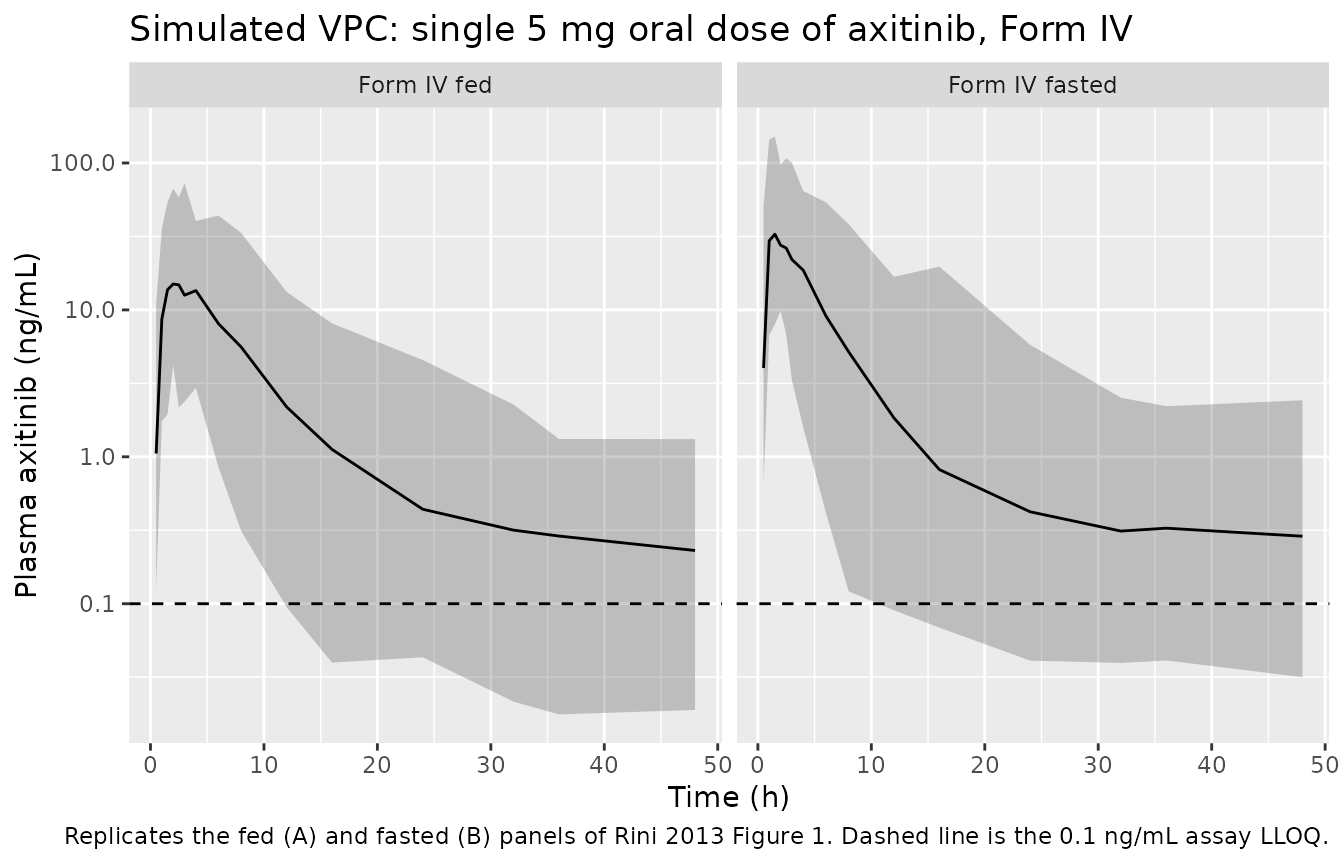
Figure 1 shows visual predictive checks of Form IV in fed (panel A)
and fasted (panel B) subjects, plotting the 2.5th, 50th and 97.5th
percentiles down to the lower limit of quantification of 0.1 ng/mL
(Methods “PK Assessment”: the assay linear range was 0.1-25 ng/mL in the
studies contributing the bulk of the single-dose data). Observed data
are not publicly distributed, so the panel below reproduces the
simulated percentile bands from the packaged model. The bands are
computed from the sim column, which carries the 58.2% oral
residual error on top of the interindividual variability, so they are
comparable to percentiles of observed concentrations rather than of
individual predictions.
lloq <- 0.1

sd_sim |>
  dplyr::filter(time > 0, treatment != "Form XLI fed") |>
  dplyr::group_by(treatment, time) |>
  dplyr::summarise(
    Q025 = stats::quantile(sim, 0.025, na.rm = TRUE),
    Q50  = stats::quantile(sim, 0.500, na.rm = TRUE),
    Q975 = stats::quantile(sim, 0.975, na.rm = TRUE),
    .groups = "drop"
  ) |>
  ggplot(aes(time, Q50)) +
  geom_ribbon(aes(ymin = Q025, ymax = Q975), alpha = 0.25) +
  geom_line() +
  geom_hline(yintercept = lloq, linetype = "dashed") +
  facet_wrap(~ treatment) +
  scale_y_log10() +
  labs(
    x = "Time (h)",
    y = "Plasma axitinib (ng/mL)",
    title = "Simulated VPC: single 5 mg oral dose of axitinib, Form IV",
    caption = paste(
      "Replicates the fed (A) and fasted (B) panels of Rini 2013 Figure 1.",
      "Dashed line is the 0.1 ng/mL assay LLOQ."
    )
  )
Single-dose NCA
sd_nca_conc <- sd_sim |>
  dplyr::filter(!is.na(Cc)) |>
  dplyr::select(id, time, Cc, treatment) |>
  as.data.frame()

sd_nca_dose <- sd_events |>
  dplyr::filter(evid == 1L) |>
  dplyr::select(id, time, amt, treatment) |>
  as.data.frame()

sd_conc_obj <- PKNCA::PKNCAconc(sd_nca_conc, Cc ~ time | treatment + id,
                                concu = "ng/mL", timeu = "h")
sd_dose_obj <- PKNCA::PKNCAdose(sd_nca_dose, amt ~ time | treatment + id, doseu = "mg")

sd_intervals <- data.frame(
  start     = 0,
  end       = 48,
  cmax      = TRUE,
  tmax      = TRUE,
  auclast   = TRUE,
  half.life = TRUE
)

sd_nca <- PKNCA::pk.nca(PKNCA::PKNCAdata(sd_conc_obj, sd_dose_obj, intervals = sd_intervals))

sd_summary <- as.data.frame(sd_nca$result) |>
  dplyr::filter(PPTESTCD %in% c("cmax", "tmax", "auclast", "half.life")) |>
  dplyr::group_by(treatment, PPTESTCD) |>
  dplyr::summarise(median_value = stats::median(PPORRES, na.rm = TRUE), .groups = "drop") |>
  tidyr::pivot_wider(names_from = PPTESTCD, values_from = median_value)

knitr::kable(
  sd_summary |>
    dplyr::rename(
      "Treatment"           = treatment,
      "AUC0-48 (h*ng/mL)"   = auclast,
      "Cmax (ng/mL)"        = cmax,
      "t1/2 (h)"            = half.life,
      "Tmax (h)"            = tmax
    ),
  digits  = 3,
  caption = "Simulated single-dose median NCA parameters by food / polymorph condition."
)| Treatment | AUC0-48 (h*ng/mL) | Cmax (ng/mL) | t1/2 (h) | Tmax (h) |
|---|---|---|---|---|
| Form IV fasted | 169.723 | 35.087 | 78.506 | 1.5 |
| Form IV fed | 123.855 | 17.462 | 70.992 | 2.5 |
| Form XLI fed | 107.246 | 15.490 | 67.216 | 2.5 |
Rini 2013 does not tabulate single-dose NCA values, but the exposure
ratios between these three arms are determined entirely by the Table 2
bioavailability effects, because CL is unchanged across the
arms:
-
AUC(Form IV fasted) / AUC(Form IV fed) = 1 + 0.330 = 1.330(Table 2 “Fasting on F, Form IV”, footnote f). -
AUC(Form XLI fed) / AUC(Form IV fed) = 1 - 0.121 = 0.879(Table 2 “Form XLI on F”, footnote g).
ka does not enter the AUC ratio, so any deviation
isolates a bioavailability transcription error. The ratio is asserted on
a typical-value (random-effects-zeroed) run rather than
on the cohort medians above: the three stochastic arms draw independent
random effects, so a ratio of their medians carries roughly 10% Monte
Carlo noise and could not support a tight bound. On the typical-value
run the only residual is the small part of the profile lying beyond the
48 h window, which the faster fasted absorption shifts slightly.
ratio_arms <- tibble::tribble(
  ~treatment,       ~FED, ~FORM_AXI_XLI,
  "Form IV fed",    1L,   0L,
  "Form IV fasted", 0L,   0L,
  "Form XLI fed",   1L,   1L
) |>
  dplyr::mutate(id = dplyr::row_number(), WT = 74.1, AGE_GT60 = 0L,
                RACE_JAPANESE = 0L, SMOKE = 0L)

ratio_obs <- c(0, seq(0.25, 12, by = 0.25), seq(13, 48, by = 1))

ratio_events <- dplyr::bind_rows(
  ratio_arms |> dplyr::mutate(time = 0, evid = 1L, amt = 5, cmt = "depot"),
  tidyr::expand_grid(id = ratio_arms$id, time = ratio_obs) |>
    dplyr::left_join(ratio_arms, by = "id") |>
    dplyr::mutate(evid = 0L, amt = 0, cmt = "central")
) |>
  dplyr::arrange(id, time, dplyr::desc(evid))

ratio_sim <- rxode2::rxSolve(mod_typ, events = as.data.frame(ratio_events),
                             keep = "treatment") |>
  as.data.frame() |>
  dplyr::mutate(id = as.integer(as.character(id)))
#> ℹ omega/sigma items treated as zero: 'etalcl', 'etalvc', 'etalq_lvp', 'etalka'
#> Warning: multi-subject simulation without without 'omega'

ratio_nca <- PKNCA::pk.nca(PKNCA::PKNCAdata(
  PKNCA::PKNCAconc(
    ratio_sim |> dplyr::filter(!is.na(Cc)) |>
      dplyr::select(id, time, Cc, treatment) |> as.data.frame(),
    Cc ~ time | treatment + id, concu = "ng/mL", timeu = "h"
  ),
  PKNCA::PKNCAdose(
    ratio_events |> dplyr::filter(evid == 1L) |>
      dplyr::select(id, time, amt, treatment) |> as.data.frame(),
    amt ~ time | treatment + id, doseu = "mg"
  ),
  intervals = data.frame(start = 0, end = 48, auclast = TRUE)
))

auc_by_arm <- as.data.frame(ratio_nca$result) |>
  dplyr::filter(PPTESTCD == "auclast") |>
  dplyr::select(treatment, PPORRES) |>
  tibble::deframe()

auc_ratio_table <- tibble::tibble(
  Ratio = c("Form IV fasted / Form IV fed", "Form XLI fed / Form IV fed"),
  `Simulated AUC0-48 ratio` = c(
    unname(auc_by_arm[["Form IV fasted"]] / auc_by_arm[["Form IV fed"]]),
    unname(auc_by_arm[["Form XLI fed"]]   / auc_by_arm[["Form IV fed"]])
  ),
  `Published F ratio (Table 2)` = c(1 + 0.330, 1 - 0.121)
) |>
  dplyr::mutate(`% difference` = 100 * (`Simulated AUC0-48 ratio` /
                                          `Published F ratio (Table 2)` - 1))

knitr::kable(
  auc_ratio_table,
  digits  = 4,
  caption = "Typical-value AUC0-48 ratios vs the published bioavailability ratios (Rini 2013 Table 2)."
)| Ratio | Simulated AUC0-48 ratio | Published F ratio (Table 2) | % difference |
|---|---|---|---|
| Form IV fasted / Form IV fed | 1.3323 | 1.330 | 0.174 |
| Form XLI fed / Form IV fed | 0.8790 | 0.879 | 0.000 |
stopifnot(
  # Form XLI shares the fed absorption profile with the Form IV reference,
  # so its AUC ratio is the F ratio exactly.
  abs(auc_ratio_table$`% difference`[2]) < 0.5,
  # The fasted arm differs in ka as well, so only the 48 h window truncation
  # separates it from the F ratio.
  abs(auc_ratio_table$`% difference`[1]) < 5
)
The Cmax and Tmax columns carry the ka effect that AUC
does not: the fasted arm’s ka of 1.43 /h (Table 2 footnote
e) versus 0.482 /h fed moves the peak earlier and higher.
tmax_by_arm <- as.data.frame(sd_nca$result) |>
  dplyr::filter(PPTESTCD == "tmax") |>
  dplyr::group_by(treatment) |>
  dplyr::summarise(median_tmax = stats::median(PPORRES), .groups = "drop")

knitr::kable(
  tmax_by_arm |> dplyr::rename("Treatment" = treatment, "Median Tmax (h)" = median_tmax),
  digits  = 2,
  caption = "Median simulated Tmax: the fasted arm peaks earlier because ka is 197% higher."
)| Treatment | Median Tmax (h) |
|---|---|
| Form IV fasted | 1.5 |
| Form IV fed | 2.5 |
| Form XLI fed | 2.5 |
stopifnot(
  # Directional: faster absorption when fasted must move the peak earlier.
  tmax_by_arm$median_tmax[tmax_by_arm$treatment == "Form IV fasted"] <
    tmax_by_arm$median_tmax[tmax_by_arm$treatment == "Form IV fed"]
)
Virtual cohort: mRCC patients at steady state
The exposure-response analysis used the 168 evaluable patients of the three mRCC studies. Their per-study design is taken from Table 1:
| Study | Population | Regimen | Enrolled |
|---|---|---|---|
| 2 | Cytokine-refractory mRCC | 5 mg bid, fasted, Form IV, dose titration | 52 |
| 4 | Sorafenib-refractory mRCC | 5 mg bid, fed, Form IV, dose titration | 62 |
| 5 | Japanese cytokine-refractory mRCC | 5 mg bid, fed, Form IV, dose titration | 64 |
Scaling the enrolled counts to the 168 analysed patients gives arms
of 49 / 59 / 60, and fixes the Japanese fraction at 60/168 = 36%, which
the paper never states directly for this subset. Median age in the
subset is exactly 60 years (Table 3), so half the cohort is assigned
AGE_GT60 = 1. No smokers are simulated (3% of the pooled PK
dataset; Rini 2013 itself excluded the smoking effect from its
covariate-impact simulations because the estimate was too
imprecise).
set.seed(20130502)

mrcc_design <- tibble::tribble(
  ~study,                                       ~n,  ~FED, ~RACE_JAPANESE,
  "Study 2 (cytokine-refractory, fasted)",      49L, 0L,   0L,
  "Study 4 (sorafenib-refractory, fed)",        59L, 1L,   0L,
  "Study 5 (Japanese cytokine-refractory, fed)", 60L, 1L,   1L
)

mrcc_cov <- mrcc_design |>
  tidyr::uncount(n) |>
  dplyr::mutate(
    id           = dplyr::row_number(),
    WT           = pmax(40, rnorm(dplyr::n(), mean = 74, sd = 15)),
    AGE_GT60     = rbinom(dplyr::n(), 1, 0.5),
    SMOKE        = 0L,
    FORM_AXI_XLI = 0L,
    treatment    = "5 mg bid, steady state"
  )

n_days   <- 28L                                   # 4 weeks of treatment, per Table 3
tau      <- 12
dose_t   <- seq(0, 24 * n_days - tau, by = tau)
ss_lo    <- 24 * n_days - 24                      # the 24 h window contains 24/tau = 2 doses
ss_hi    <- 24 * n_days
obs_t    <- seq(ss_lo, ss_hi, by = 0.1)

mrcc_events <- dplyr::bind_rows(
  tidyr::expand_grid(id = mrcc_cov$id, time = dose_t) |>
    dplyr::left_join(mrcc_cov, by = "id") |>
    dplyr::mutate(evid = 1L, amt = 5, cmt = "depot"),
  tidyr::expand_grid(id = mrcc_cov$id, time = obs_t) |>
    dplyr::left_join(mrcc_cov, by = "id") |>
    dplyr::mutate(evid = 0L, amt = 0, cmt = "central")
) |>
  dplyr::arrange(id, time, dplyr::desc(evid))

stopifnot(nrow(mrcc_cov) == 168L)
mrcc_sim <- rxode2::rxSolve(
  mod,
  events = as.data.frame(mrcc_events),
  keep   = c("study", "treatment")
) |>
  as.data.frame() |>
  dplyr::mutate(id = as.integer(as.character(id)))
Steady-state NCA and the AUC identity
For a linear model at steady state, the AUC over one dosing interval
is exactly dose * F / CL, so the AUC over the 24 h window
(which contains both daily doses) is exactly
total daily dose * F / CL – the quantity Rini 2013 Methods
“PK/PD Modeling” defines as the mean daily AUC. Both sides of the check
below use the same drawn parameters, so the only sources of difference
are trapezoidal error and the small residual approach to steady state
after 28 days.
mrcc_nca_conc <- mrcc_sim |>
  dplyr::filter(!is.na(Cc)) |>
  dplyr::select(id, time, Cc, treatment) |>
  as.data.frame()

# Only the two doses inside the analysis window are passed to PKNCA; the 54
# earlier doses have no concentration records and would put the AUC interval
# before the first measurement.
mrcc_nca_dose <- mrcc_events |>
  dplyr::filter(evid == 1L, time >= ss_lo) |>
  dplyr::select(id, time, amt, treatment) |>
  as.data.frame()

mrcc_conc_obj <- PKNCA::PKNCAconc(mrcc_nca_conc, Cc ~ time | treatment + id,
                                  concu = "ng/mL", timeu = "h")
mrcc_dose_obj <- PKNCA::PKNCAdose(mrcc_nca_dose, amt ~ time | treatment + id, doseu = "mg")

mrcc_intervals <- data.frame(
  start   = ss_lo,
  end     = ss_hi,
  cmax    = TRUE,
  cmin    = TRUE,
  auclast = TRUE,
  cav     = TRUE
)

mrcc_nca <- PKNCA::pk.nca(
  PKNCA::PKNCAdata(mrcc_conc_obj, mrcc_dose_obj, intervals = mrcc_intervals)
)

# Per-subject individual parameters carried out of the solve.
mrcc_pars <- mrcc_sim |>
  dplyr::group_by(id) |>
  dplyr::slice_head(n = 1) |>
  dplyr::ungroup() |>
  dplyr::select(id, study, cl, fdepot) |>
  dplyr::mutate(id = as.integer(as.character(id)))

auc_check <- as.data.frame(mrcc_nca$result) |>
  dplyr::filter(PPTESTCD == "auclast") |>
  dplyr::select(id, auc24_nca = PPORRES) |>
  dplyr::mutate(id = as.integer(as.character(id))) |>
  dplyr::left_join(mrcc_pars, by = "id") |>
  dplyr::mutate(
    # 10 mg total daily dose, mg / (L/h) -> mg*h/L, scaled to ng*h/mL.
    auc24_identity = 10 * fdepot / cl * 1000,
    pct_diff       = 100 * (auc24_nca - auc24_identity) / auc24_identity
  )

knitr::kable(
  tibble::tibble(
    Statistic = c("Median % difference", "90th percentile of |% difference|",
                  "Maximum |% difference|"),
    Value     = c(stats::median(auc_check$pct_diff),
                  unname(stats::quantile(abs(auc_check$pct_diff), 0.9)),
                  max(abs(auc_check$pct_diff)))
  ),
  digits  = 2,
  caption = "Simulated steady-state AUC0-24 vs the closed-form identity total daily dose * F / CL."
)| Statistic | Value |
|---|---|
| Median % difference | -0.21 |
| 90th percentile of |% difference| | 3.20 |
| Maximum |% difference| | 37.04 |
stopifnot(
  # Structural: a mis-transcribed CL, F or dose moves the whole distribution.
  abs(stats::median(auc_check$pct_diff)) < 2,
  # Envelope: robust to the subjects with the largest peripheral volumes,
  # which are the slowest to reach steady state after 28 days of dosing.
  stats::quantile(abs(auc_check$pct_diff), 0.9) < 8
)
Comparison against the published exposure distribution
Rini 2013 Table 3 reports a median mean-daily AUC of 375 h*ng/mL (range 32.8-1,728) for the 168 patients at the end of 4 weeks of treatment. Two simulated quantities are shown against it.
The published-formula AUC applies the paper’s own
equation using a single population mean F for every
patient, as Methods “PK/PD Modeling” specifies (“the population mean
estimate of F”), with the Form IV fed value 0.457. The
model-simulated AUC0-24 instead uses each patient’s own
record-level F, which is 33% higher for the fasted study 2
arm; it is the model’s prediction of true exposure and is therefore
expected to sit above the published number.
auc_check <- auc_check |>
  dplyr::mutate(auc24_paper_formula = 10 * 0.457 / cl * 1000)

auc_compare <- tibble::tibble(
  Quantity = c("Published-formula AUC (single population F = 0.457)",
               "Model-simulated steady-state AUC0-24 (record-level F)"),
  `Simulated median (h*ng/mL)` = c(stats::median(auc_check$auc24_paper_formula),
                                   stats::median(auc_check$auc24_nca)),
  `Published median (h*ng/mL)` = 375
) |>
  dplyr::mutate(`% difference` = 100 * (`Simulated median (h*ng/mL)` /
                                          `Published median (h*ng/mL)` - 1))

knitr::kable(
  auc_compare,
  digits  = 1,
  caption = "Simulated vs published median mean-daily AUC in the 168-patient mRCC subset (Rini 2013 Table 3)."
)| Quantity | Simulated median (h*ng/mL) | Published median (h*ng/mL) | % difference |
|---|---|---|---|
| Published-formula AUC (single population F = 0.457) | 417.1 | 375 | 11.2 |
| Model-simulated steady-state AUC0-24 (record-level F) | 427.3 | 375 | 14.0 |
stopifnot(
  # The paper's own AUC formula, evaluated on the model's individual
  # clearances, must land near the published median. This is a comparison of
  # cohort medians, not of extremes, so it is stable across rxode2 builds.
  abs(stats::median(auc_check$auc24_paper_formula) / 375 - 1) < 0.25
)
Per-study medians show where the pooled difference comes from: the fasted study 2 arm carries the 33% bioavailability increase, and the Japanese study 5 arm carries the 24.9% clearance reduction.
auc_by_study <- auc_check |>
  dplyr::group_by(study) |>
  dplyr::summarise(
    n                     = dplyr::n(),
    median_auc24_nca      = stats::median(auc24_nca),
    median_auc24_formula  = stats::median(auc24_paper_formula),
    .groups = "drop"
  )

knitr::kable(
  auc_by_study |>
    dplyr::rename(
      "Study"                                       = study,
      "n"                                           = n,
      "Median simulated AUC0-24 (h*ng/mL)"          = median_auc24_nca,
      "Median published-formula AUC (h*ng/mL)"      = median_auc24_formula
    ),
  digits  = 1,
  caption = "Simulated mean-daily exposure by mRCC study arm."
)| Study | n | Median simulated AUC0-24 (h*ng/mL) | Median published-formula AUC (h*ng/mL) |
|---|---|---|---|
| Study 2 (cytokine-refractory, fasted) | 49 | 492.0 | 370.1 |
| Study 4 (sorafenib-refractory, fed) | 59 | 372.0 | 372.7 |
| Study 5 (Japanese cytokine-refractory, fed) | 60 | 497.3 | 500.7 |
Replicating Supplementary Figure S4
Supplementary Figure S4 shows axitinib AUC12 for a
typical fed subject in each of four covariate cells – age > 60 or
not, Japanese or not – receiving 5 mg Form XLI twice daily. The four
typical values are exactly
5 mg * F(Form XLI) / CL(covariates), so the model
reproduces the figure’s structure in closed form. The figure itself
plots medians and 95% prediction intervals as an image, so only the
ratios are checked here.
fig_s4 <- tidyr::expand_grid(
  AGE_GT60      = c(0L, 1L),
  RACE_JAPANESE = c(0L, 1L)
) |>
  dplyr::mutate(
    id        = dplyr::row_number(),
    WT        = 74.1,
    SMOKE     = 0L,
    FED       = 1L,
    FORM_AXI_XLI = 1L,
    group     = paste0(ifelse(AGE_GT60 == 1L, ">60 y", "<=60 y"), ", ",
                       ifelse(RACE_JAPANESE == 1L, "Japanese", "non-Japanese"))
  )

fig_s4_events <- dplyr::bind_rows(
  fig_s4 |> dplyr::mutate(time = 0, evid = 1L, amt = 5, cmt = "depot"),
  fig_s4 |> dplyr::mutate(time = 1, evid = 0L, amt = 0, cmt = "central")
) |>
  dplyr::arrange(id, time, dplyr::desc(evid))

fig_s4_par <- rxode2::rxSolve(
  mod_typ,
  events = as.data.frame(fig_s4_events),
  keep   = "group"
) |>
  as.data.frame() |>
  dplyr::group_by(group) |>
  dplyr::slice_head(n = 1) |>
  dplyr::ungroup() |>
  # rxSolve returns the covariate columns alongside the model variables.
  dplyr::select(group, AGE_GT60, RACE_JAPANESE, cl, fdepot) |>
  dplyr::mutate(auc12 = 5 * fdepot / cl * 1000) |>
  dplyr::arrange(AGE_GT60, RACE_JAPANESE)
#> ℹ omega/sigma items treated as zero: 'etalcl', 'etalvc', 'etalq_lvp', 'etalka'
#> Warning: multi-subject simulation without without 'omega'

ref_auc12 <- fig_s4_par$auc12[fig_s4_par$AGE_GT60 == 0L & fig_s4_par$RACE_JAPANESE == 0L]

fig_s4_par <- fig_s4_par |>
  dplyr::mutate(
    ratio_vs_reference = auc12 / ref_auc12,
    expected_ratio     = 1 / ((1 - 0.213 * AGE_GT60) * (1 - 0.249 * RACE_JAPANESE))
  )

knitr::kable(
  fig_s4_par |>
    dplyr::select(group, auc12, ratio_vs_reference, expected_ratio) |>
    dplyr::rename(
      "Covariate cell"                        = group,
      "Typical AUC12 (h*ng/mL)"               = auc12,
      "Ratio vs <=60 y non-Japanese"          = ratio_vs_reference,
      "Expected from Table 2 CL effects"      = expected_ratio
    ),
  digits  = 3,
  caption = "Typical AUC12 for the four Supplementary Figure S4 covariate cells, 5 mg bid Form XLI fed."
)| Covariate cell | Typical AUC12 (h*ng/mL) | Ratio vs <=60 y non-Japanese | Expected from Table 2 CL effects |
|---|---|---|---|
| <=60 y, non-Japanese | 137.570 | 1.000 | 1.000 |
| <=60 y, Japanese | 183.182 | 1.332 | 1.332 |
| >60 y, non-Japanese | 174.802 | 1.271 | 1.271 |
| >60 y, Japanese | 232.760 | 1.692 | 1.692 |
stopifnot(isTRUE(all.equal(fig_s4_par$ratio_vs_reference,
                           fig_s4_par$expected_ratio, tolerance = 1e-8)))
Rini 2013 concludes from this simulation that “the magnitude of predicted changes in exposure based on these covariates does not warrant dose adjustments” (Abstract). The largest cell – an over-60 Japanese subject – has a typical exposure 1.69 times the reference, which is far smaller than the 59.9% CV of clearance itself, exactly as the Discussion argues.
Body weight moves Cmax but not exposure
Rini 2013 Results “Effects of covariates” states that “expected
changes in peak plasma concentrations due to body weight were less than
the estimated IIV for Vc” and, crucially, that “exposure is not affected
by changes in Vc”. Because weight acts only on Vc, the
steady-state AUC identity is weight-independent while Cmax is not – a
check the model must pass exactly.
wt_grid <- tibble::tibble(
  WT    = c(58, 74.1, 94),                            # 10th percentile, median, 90th percentile
  label = c("58 kg (10th percentile)", "74.1 kg (median)", "94 kg (90th percentile)")
) |>
  dplyr::mutate(id = dplyr::row_number(), AGE_GT60 = 0L, RACE_JAPANESE = 0L,
                SMOKE = 0L, FED = 1L, FORM_AXI_XLI = 1L)

wt_events <- dplyr::bind_rows(
  tidyr::expand_grid(id = wt_grid$id, time = dose_t) |>
    dplyr::left_join(wt_grid, by = "id") |>
    dplyr::mutate(evid = 1L, amt = 5, cmt = "depot"),
  tidyr::expand_grid(id = wt_grid$id, time = obs_t) |>
    dplyr::left_join(wt_grid, by = "id") |>
    dplyr::mutate(evid = 0L, amt = 0, cmt = "central")
) |>
  dplyr::arrange(id, time, dplyr::desc(evid))

wt_solved <- rxode2::rxSolve(mod_typ, events = as.data.frame(wt_events), keep = "label") |>
  as.data.frame() |>
  dplyr::mutate(id = as.integer(as.character(id)))
#> ℹ omega/sigma items treated as zero: 'etalcl', 'etalvc', 'etalq_lvp', 'etalka'
#> Warning: multi-subject simulation without without 'omega'

wt_nca <- PKNCA::pk.nca(PKNCA::PKNCAdata(
  PKNCA::PKNCAconc(
    wt_solved |> dplyr::filter(!is.na(Cc)) |>
      dplyr::select(id, time, Cc, label) |> as.data.frame(),
    Cc ~ time | label + id, concu = "ng/mL", timeu = "h"
  ),
  PKNCA::PKNCAdose(
    wt_events |> dplyr::filter(evid == 1L, time >= ss_lo) |>
      dplyr::select(id, time, amt, label) |> as.data.frame(),
    amt ~ time | label + id, doseu = "mg"
  ),
  intervals = data.frame(start = ss_lo, end = ss_hi,
                         cmax = TRUE, cmin = TRUE, auclast = TRUE)
))

wt_sim <- as.data.frame(wt_nca$result) |>
  dplyr::filter(PPTESTCD %in% c("cmax", "cmin", "auclast")) |>
  dplyr::select(label, PPTESTCD, PPORRES) |>
  tidyr::pivot_wider(names_from = PPTESTCD, values_from = PPORRES) |>
  dplyr::rename(cmax_ss = cmax, cmin_ss = cmin, auc24 = auclast) |>
  dplyr::arrange(match(label, wt_grid$label))

knitr::kable(
  wt_sim |>
    dplyr::rename(
      "Body weight"            = label,
      "Cmax,ss (ng/mL)"        = cmax_ss,
      "Cmin,ss (ng/mL)"        = cmin_ss,
      "AUC0-24,ss (h*ng/mL)"   = auc24
    ),
  digits  = 2,
  caption = "Typical-value steady-state exposure at three body weights, 5 mg bid Form XLI fed."
)| Body weight | AUC0-24,ss (h*ng/mL) | Cmax,ss (ng/mL) | Cmin,ss (ng/mL) |
|---|---|---|---|
| 58 kg (10th percentile) | 274.84 | 21.87 | 3.41 |
| 74.1 kg (median) | 274.83 | 20.28 | 3.84 |
| 94 kg (90th percentile) | 274.83 | 18.89 | 4.36 |
As an external cross-check, the companion healthy-volunteer analysis (Garrett 2014 Results “Full model and final model”) publishes typical steady-state Cmax values for exactly this regimen at three body weights: 20.6 ng/mL at 62 kg, 19.3 ng/mL at 75 kg and 17.9 ng/mL at 93 kg. The Rini 2013 model reproduces the same magnitude and the same weight trend from an independently estimated parameter set. That is corroboration across two papers, not a Rini 2013 claim, so it is not asserted.
stopifnot(
  # AUC is weight-independent: identical to well within trapezoidal error.
  diff(range(wt_sim$auc24)) / stats::median(wt_sim$auc24) < 0.005,
  # Cmax decreases with weight, because Vc increases with weight.
  wt_sim$cmax_ss[wt_sim$label == "58 kg (10th percentile)"] >
    wt_sim$cmax_ss[wt_sim$label == "94 kg (90th percentile)"]
)
Exposure-response linkage
The Cox and logistic regression models of Rini 2013 are not encoded in the model file (see Errata), but the packaged PK model supplies the exposure metric they take as input, so the published coefficients can be applied to the simulated cohort to reproduce the paper’s relative statements. Table 5 gives, after adjustment for gender, prior therapy, ECOG PS and haemoglobin, a hazard ratio of 0.909 per 100 h*ng/mL of AUC for progression-free survival and 0.866 for overall survival.
auc_iqr <- stats::quantile(auc_check$auc24_paper_formula, c(0.25, 0.75))

hr_table <- tibble::tibble(
  Endpoint = c("Progression-free survival", "Overall survival"),
  `HR per 100 h*ng/mL (Table 5)` = c(0.909, 0.866),
  `HR across the simulated interquartile AUC range` =
    c(0.909, 0.866)^(unname(diff(auc_iqr)) / 100)
)

knitr::kable(
  hr_table,
  digits  = 3,
  caption = sprintf(
    paste("Published Table 5 hazard ratios applied across the simulated",
          "interquartile AUC range (%.0f to %.0f h*ng/mL)."),
    auc_iqr[1], auc_iqr[2]
  )
)| Endpoint | HR per 100 h*ng/mL (Table 5) | HR across the simulated interquartile AUC range |
|---|---|---|
| Progression-free survival | 0.909 | 0.715 |
| Overall survival | 0.866 | 0.603 |
Rini 2013 also stratified patients at 300 h*ng/mL, reporting 38% of the 168 patients below the cutoff and 62% at or above it (Table 3). The simulated cohort’s split is shown below. The paper’s split is computed from post-hoc empirical Bayes clearances at the patients’ actual (sometimes reduced) daily doses, while the simulation holds every patient at 5 mg twice daily, so the simulated fraction above the cutoff is expected to be somewhat higher.
cutoff_table <- tibble::tibble(
  Group = c("AUC < 300 h*ng/mL", "AUC >= 300 h*ng/mL"),
  `Simulated %` = c(
    100 * mean(auc_check$auc24_paper_formula <  300),
    100 * mean(auc_check$auc24_paper_formula >= 300)
  ),
  `Published % (Table 3)` = c(38, 62)
)

knitr::kable(cutoff_table, digits = 1,
caption = "Distribution around the 300 h*ng/mL exposure cutoff of Rini 2013 Table 3.")| Group | Simulated % | Published % (Table 3) |
|---|---|---|
| AUC < 300 h*ng/mL | 32.1 | 38 |
| AUC >= 300 h*ng/mL | 67.9 | 62 |
Assumptions and deviations
-
Interindividual variability scale. Rini 2013 Table
2 footnote a reports the IIV as “%CV” without stating the
back-transformation. The packaged model takes
omega^2 = (%CV / 100)^2, following the convention used by the same modelling group in the companion healthy-volunteer analysis (Garrett 2014), whose Methods print the definition verbatim –%IIV = sqrt(omega^2) x 100– and whose Table 3 satisfies it numerically:omega^2(Vc) = 0.0949givessqrt(0.0949) = 30.8%, exactly the 30.8% Vc IIV that paper’s Discussion quotes, whereas the exact-log-normal back-transformation would give 31.6% and does not match. The alternative reading –%CVas the exact log-normal coefficient of variation,omega^2 = log(1 + CV^2)– would giveomega = 0.657rather than0.599for clearance, about 10% larger. The choice changes only the width of the simulated distributions; it changes no typical value, no covariate effect, and none of the structural identities checked above. It does slightly widen or narrow the VPC bands of Figure 1 and the 95% prediction intervals of Supplementary Figures S4 and S5. -
Route-stratified residual error not encoded. Rini
2013 fit two residuals on the log-concentration scale – oral 58.2% and
intravenous 33.5% (Table 2). The packaged model encodes a single
expSd = 0.582, the oral value, because a single rxode2 endpoint carries a single error model and the library use of this model is oral dosing; the intravenous arm existed only to anchor absolute bioavailability (16 subjects, study 8). Users simulating the intravenous arm should overrideexpSd <- 0.335afterreadModelDb(). -
Residual error form. Methods “Model development”
states that log-transformed concentrations were modelled with a
proportional residual. An additive residual on the log-concentration
scale is a log-normal residual on the linear scale, which is how it is
encoded (
Cc ~ lnorm(expSd)); at 58.2% the log-normal and the linear-scale proportional forms are not interchangeable, and the log-scale reading is the one the Methods sentence supports. -
Fasting effect on F is gated to Form IV. Table 2’s
row label is “Fasting on F, Form IV” and footnote g states explicitly
that “there was no observed food effect with Form XLI”, giving
F = 0.402for Form XLI in either prandial state. The model therefore multiplies the fasting term by(1 - FORM_AXI_XLI). The fasting effect onka, by contrast, is applied to both polymorphs, because Results “Effects of covariates” says it holds “regardless of formulations”. -
Q and Vp share one random effect. Table 2 footnote
d states that Q and Vp were modelled as 100% correlated with the same
interindividual variability. That is encoded as a single shared
etalq_lvprather than a 2x2 block with unit correlation, which would be singular and would fail Cholesky decomposition at simulation time. -
Covariate distributions of the virtual cohorts are
assumptions. Rini 2013 reports no per-subject covariate table.
Body weight is drawn as
Normal(74, 15)truncated below at 40 kg to match the reported median 74 kg and range 37-136 kg; the mRCC cohort’sAGE_GT60is drawn at 50% because the subset’s median age is exactly 60 years (Table 3); the Japanese fraction of 36% is derived from Table 1 (study 5 contributed 64 of the 178 enrolled mRCC patients); no smokers are simulated. Weight is immaterial to every exposure comparison here, because it acts only onVc. - Steady state is approached, not reached exactly. The peripheral volume of 393 L against an inter-compartmental clearance of 4.00 L/h gives a long, low-amplitude terminal phase, so 28 days of 5 mg bid dosing leaves a small accumulation deficit. That is the entire content of the median -0.2% and 90th-percentile 2.5% deviations in the AUC identity check; the subjects furthest from steady state are those whose shared Q / Vp random effect gave them the largest peripheral volume. Twenty-eight days matches the paper’s own “end of 4 weeks of study treatment” exposure window.
- Dose titration is not simulated. Patients could titrate to 10 mg bid or have doses reduced or interrupted for hypertension, and Rini 2013 computed each patient’s AUC from their “average total daily dose”. The simulated cohort holds every patient at 5 mg bid, which is what the paper describes as the situation at the end of 4 weeks “prior to dose changes in most patients”.
-
VPC bands are simulated only. The Figure 1
replication plots percentiles of the
simcolumn, which carries both interindividual and the 58.2% oral residual variability, so it is the right analogue of the published observed-percentile bands. What it cannot reproduce is the observed data themselves, or the published bands’ truncation at the 0.1 ng/mL LLOQ; the LLOQ is drawn as a reference line instead. The NCA blocks useCc(individual predictions without residual error), which is what makes the structural AUC identities exact.
Errata and unencoded sub-models
-
No erratum located. A search of the journal’s
correction notices and of PubMed for corrections to
doi:10.1002/jcph.73returned nothing; no erratum is referenced by the article record. - The Cox proportional-hazards models are not encoded. Rini 2013 Table 5 reports regression coefficients and hazard ratios for progression-free and overall survival as functions of AUC, diastolic blood pressure, gender, prior therapy, ECOG PS and haemoglobin, but it reports no baseline hazard function and no baseline survival curve. A Cox model’s partial likelihood does not estimate the baseline hazard, so a semi-parametric fit reported this way cannot be turned into a simulatable time-to-event model without information the paper does not contain. The published coefficients are applied above as relative statements, which is all they support.
- The logistic regression models are not encoded. Rini 2013 reports only the odds-ratio slopes – a 1.5-fold increase in the probability of a partial response per 100 h*ng/mL of AUC, and 1.6-fold per 10 mm Hg of diastolic blood pressure – and marks the underlying fits as “data not shown”. Without an intercept the absolute response probability is not recoverable.
-
No diastolic blood pressure model. Diastolic blood
pressure enters the paper only as an observed covariate in the
regression analyses. Rini 2013 reports a weak relationship between
exposure and blood pressure (
r^2 < 0.10, “data not shown”) and no structural pharmacodynamic model linking axitinib concentration to blood pressure. - Base-model IIV values are prose-only. The Discussion reports that the covariate model reduced CL IIV from 64% to 60% and Vc IIV from 44% to 40%. The base model is not otherwise tabulated and is not packaged.