Moxifloxacin bone penetration (Landersdorfer 2009)
Source:vignettes/articles/Landersdorfer_2009_moxifloxacin.Rmd
Landersdorfer_2009_moxifloxacin.RmdModel and source
- Citation: Landersdorfer CB, Kinzig M, Hennig FF, Bulitta JB, Holzgrabe U, Drusano GL, Sorgel F, Gusinde J. Penetration of moxifloxacin into bone evaluated by Monte Carlo simulation. Antimicrob Agents Chemother. 2009 May;53(5):2074-81. doi:10.1128/AAC.01056-08. PMID 19237653.
- Description: Population PK model for oral moxifloxacin bone penetration (Landersdorfer 2009): two-compartment plasma disposition with first-order absorption from a gut depot, plus two paper-mechanistic bone matrix compartments (cortical and cancellous bone) connected to the central compartment by fixed transfer rate constants. The bone tissue:serum equilibrium concentration ratio is captured by the multiplicative scale terms fcortical and fcancellous on the cortical and cancellous bone observations. Disposition parameters were MAP-Bayesian estimated against Simon 1997 priors; bone-penetration scale terms used noninformative priors. Single 400 mg oral dose in 24 adults undergoing total hip replacement; serum and femoral bone samples (cortical + cancellous, head + neck) collected 2 to 7 hours post-dose.
- Article: https://doi.org/10.1128/AAC.01056-08
Population
Landersdorfer et al. enrolled 24 adults (10 men, 14 women) undergoing elective total hip replacement for coxarthrosis (no joint inflammation). Mean (SD) baseline weight was 76.8 (13.4) kg, height 168.3 (9.9) cm, and age 63 (15) years. Each patient received a single 400 mg oral dose of moxifloxacin (Avalox tablet) 2 to 7 hours before surgery. Sampling was sparse: one pre-resection serum sample and one bone sample (femoral head, with or without femoral neck; separated into cortical and cancellous tissue) per subject. Twenty patients also received intravenous amoxicillin-clavulanate, three received levofloxacin, and one received clindamycin as standard perioperative antibacterial prophylaxis. The study was performed in Germany (University of Erlangen). Demographic and sampling details are taken from Materials and Methods ‘Study participants’ and ‘Sampling schedule’. No covariate was retained on any PK parameter in the final model.
The same information is available programmatically via
readModelDb("Landersdorfer_2009_moxifloxacin")$population.
Source trace
Per-parameter origin comments are recorded in
inst/modeldb/specificDrugs/Landersdorfer_2009_moxifloxacin.R.
The table below collects them in one place.
| Equation / parameter | Value | Source location |
|---|---|---|
lka (absorption rate) |
log(1.6) | Results ‘PK analysis’ paragraph 1; absorption half-life 26 min from NONMEM V |
lcl (apparent CL/F) |
log(10.8) | Table 1 MAP-Bayesian (ADAPT II) median 10.8 L/h (range 9.85-11.5) |
lvc (apparent V_Central/F) |
log(62.0) | Table 1 MAP-Bayesian median 62.0 L (range 58.5-65.4) |
lvp (apparent V_Peripheral/F) |
log(59.5) | Table 1 MAP-Bayesian median 59.5 L (range 48.0-71.6) |
lq (apparent CL_ic/F) |
log(18.9) | Table 1 MAP-Bayesian median 18.9 L/h (range 15.3-23.2) |
lfcortical (cortical bone:serum ratio) |
log(0.803) | Table 1 MAP-Bayesian median 0.803 (35% CV, range 0.185-1.71) |
lfcancellous (cancellous bone:serum ratio) |
log(0.775) | Table 1 MAP-Bayesian median 0.775 (48% CV, range 0.278-1.56) |
etalfcortical (IIV variance) |
0.115573 | log(1 + 0.35^2); 35% CV per Table 1 |
etalfcancellous (IIV variance) |
0.207436 | log(1 + 0.48^2); 48% CV per Table 1 |
k_cb_in (k24 = k25, central -> bone) |
0.022 1/h | Materials and Methods ‘PK modeling approach’ paragraph 3 (paired with V_bone = 0.5 L) |
k_cb_out (k42 = k52, bone -> central) |
ln(2)/0.25 1/h | Materials and Methods ‘PK modeling approach’ paragraph 2; 15 min equilibration half-life |
vbone (cortical and cancellous bone volume) |
0.5 L (fixed) | Materials and Methods ‘PK modeling approach’ paragraph 3 |
d/dt(depot), d/dt(central),
d/dt(peripheral1), d/dt(cortical),
d/dt(cancellous)
|
structural ODE | Materials and Methods ‘Structural model’, Fig 1 diagram |
propSd, propSd_Ccortical,
propSd_Ccancellous
|
fixed(0) placeholders | Materials and Methods ‘MAP-Bayesian estimation’ specifies proportional residual error; numerical magnitudes not reported |
Virtual cohort
The original observed data are not publicly available. We simulate a virtual cohort whose demographics approximate the published trial (mean weight 76.8 kg, 58% female, 24 subjects per cohort for an order-of-magnitude reproduction of Figure 3’s between-subject distribution; we scale up to 1000 subjects for the simulation since the model has no covariates and the published Figure 3 itself was based on 10000 simulated subjects).
set.seed(2009L)
n_subj <- 1000L

# No covariates are used by the model; the per-subject simulation needs only an
# id and the dose record. We carry a 'dose_group' label for the PKNCA grouping
# even though all subjects receive the same regimen.
dose_amt <- 400  # mg, single oral dose

make_cohort <- function(n, id_offset = 0L) {
  obs_t <- seq(0, 36, by = 0.1)  # 36 h covers absorption + > 2 half-lives
  ids <- id_offset + seq_len(n)
  dose_rows <- data.frame(
    id   = ids,
    time = 0,
    amt  = dose_amt,
    cmt  = "depot",
    evid = 1L,
    dose_group = "400 mg PO"
  )
  obs_rows <- expand.grid(id = ids, time = obs_t) |>
    dplyr::arrange(id, time) |>
    dplyr::mutate(
      amt  = NA_real_,
      cmt  = "Cc",
      evid = 0L,
      dose_group = "400 mg PO"
    )
  dplyr::bind_rows(dose_rows, obs_rows) |>
    dplyr::arrange(id, time)
}

events <- make_cohort(n = n_subj)
stopifnot(!anyDuplicated(unique(events[, c("id", "time", "evid")])))
Simulation
The packaged model has IIV only on lfcortical and
lfcancellous (the bone tissue:serum equilibrium
concentration ratios; 35% and 48% CV per Table 1); no IIV is encoded on
the disposition parameters. See Assumptions and deviations
below. We simulate both the stochastic VPC (Figure 3 ratios) and the
typical-value profiles (Figure 2 concentration curves).
mod <- readModelDb("Landersdorfer_2009_moxifloxacin")

# Stochastic simulation: F_cortical and F_cancellous vary across subjects.
sim_stoch <- rxode2::rxSolve(mod, events = events, keep = c("dose_group"))
#> ℹ parameter labels from comments will be replaced by 'label()'

# Typical-value simulation: zero out the F-IIVs to reproduce typical curves.
mod_typ <- mod |> rxode2::zeroRe()
#> ℹ parameter labels from comments will be replaced by 'label()'
events_typ <- make_cohort(n = 1L)
sim_typ <- rxode2::rxSolve(mod_typ, events = events_typ)
#> ℹ omega/sigma items treated as zero: 'etalfcortical', 'etalfcancellous'
Replicate Figure 2: typical concentration-time profiles in serum and bone
Figure 2 of Landersdorfer 2009 plots serum, cortical bone, and cancellous bone concentrations after a single oral dose of 400 mg moxifloxacin. The typical profile below shows the same rapid equilibration of serum and bone observed in the source paper.
fig2 <- sim_typ |>
  dplyr::filter(time > 0 & time <= 24) |>
  dplyr::select(time, Serum = Cc, Cortical = Ccortical, Cancellous = Ccancellous) |>
  tidyr::pivot_longer(-time, names_to = "Matrix", values_to = "C")

ggplot(fig2, aes(time, C, colour = Matrix)) +
  geom_line(linewidth = 0.8) +
  scale_y_log10() +
  labs(x = "Time after oral dose (h)",
       y = "Moxifloxacin concentration (mg/L)",
       title = "Figure 2 - typical concentration profile, 400 mg oral",
       caption = "Replicates Figure 2 of Landersdorfer 2009 (typical-value profile).")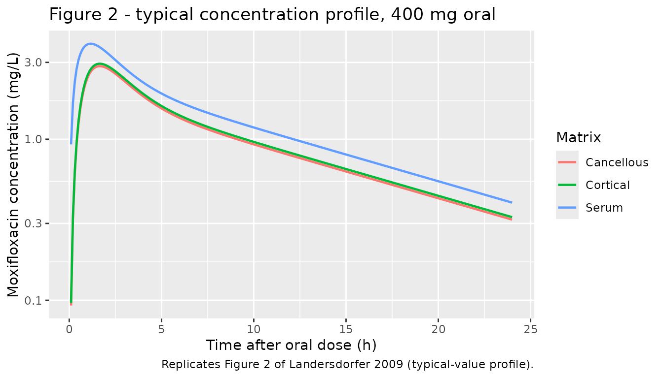
Replicate Figure 3: bone:serum AUC ratio distribution
Figure 3 of Landersdorfer 2009 shows the distribution of cortical bone:serum and cancellous bone:serum AUC ratios at steady state across 10000 simulated subjects, with the published medians and 10-90% percentiles given as:
| Matrix | Median | 10% | 90% |
|---|---|---|---|
| Cortical | 0.80 | 0.51 | 1.26 |
| Cancellous | 0.78 | 0.42 | 1.44 |
We reproduce the AUC ratios under a single 400 mg dose (the model is linear in dose, so single-dose AUC ratios equal steady-state AUC ratios under repeated q24h dosing).
tr_auc <- function(t, c) sum(diff(t) * (head(c, -1) + tail(c, -1)) / 2)

auc_by_id <- sim_stoch |>
  dplyr::filter(time > 0) |>
  dplyr::group_by(id) |>
  dplyr::summarise(
    AUC_serum      = tr_auc(time, Cc),
    AUC_cortical   = tr_auc(time, Ccortical),
    AUC_cancellous = tr_auc(time, Ccancellous),
    .groups = "drop"
  ) |>
  dplyr::mutate(
    ratio_cortical   = AUC_cortical   / AUC_serum,
    ratio_cancellous = AUC_cancellous / AUC_serum
  )

summary_tbl <- data.frame(
  Matrix = c("Cortical", "Cancellous"),
  Median = c(median(auc_by_id$ratio_cortical),    median(auc_by_id$ratio_cancellous)),
  P10    = c(quantile(auc_by_id$ratio_cortical,    0.10),
             quantile(auc_by_id$ratio_cancellous, 0.10)),
  P90    = c(quantile(auc_by_id$ratio_cortical,    0.90),
             quantile(auc_by_id$ratio_cancellous, 0.90))
)
summary_tbl_disp <- summary_tbl
summary_tbl_disp[, 2:4] <- round(summary_tbl_disp[, 2:4], 2)
knitr::kable(summary_tbl_disp,
caption = "Simulated AUC ratio distribution (n = 1000).")| Matrix | Median | P10 | P90 |
|---|---|---|---|
| Cortical | 0.80 | 0.51 | 1.22 |
| Cancellous | 0.77 | 0.43 | 1.39 |
auc_long <- auc_by_id |>
  dplyr::select(id, Cortical = ratio_cortical, Cancellous = ratio_cancellous) |>
  tidyr::pivot_longer(-id, names_to = "Matrix", values_to = "ratio")

ggplot(auc_long, aes(ratio, fill = Matrix)) +
  geom_histogram(bins = 40, alpha = 0.65, position = "identity") +
  geom_vline(xintercept = 1, linetype = "dotted") +
  facet_wrap(~Matrix, ncol = 1, scales = "free_y") +
  labs(x = "AUC_bone / AUC_serum",
       y = "Number of simulated subjects",
       title = "Figure 3 - bone:serum AUC ratio distribution",
       caption = "Replicates Figure 3 of Landersdorfer 2009; published medians 0.80 / 0.78.")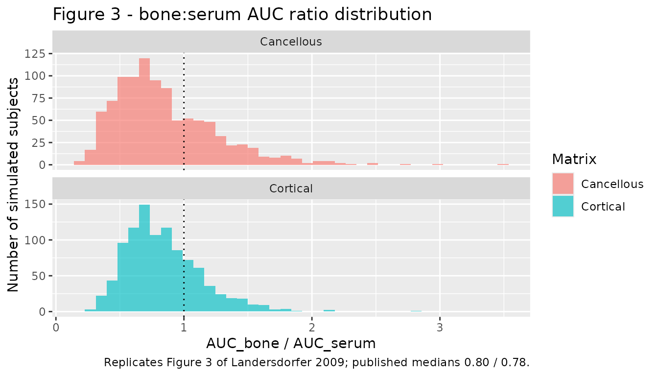
PKNCA validation
The source paper does not tabulate Cmax / Tmax for serum, but the model should produce a moxifloxacin Cmax in the ~3-4 mg/L range and AUC_inf in the ~36-37 mg.h/L range, consistent with the literature for 400 mg oral moxifloxacin (e.g., the disposition priors from Simon et al. 1997 cited by Landersdorfer 2009). We use PKNCA to compute the simulated NCA parameters on the typical-value serum curve.
sim_nca <- sim_typ |>
  dplyr::filter(time > 0 & !is.na(Cc)) |>
  dplyr::transmute(id = 1L, time = time, Cc = Cc, dose_group = "400 mg PO")

conc_obj <- PKNCA::PKNCAconc(sim_nca, Cc ~ time | dose_group + id)

dose_df <- data.frame(
  id   = 1L,
  time = 0,
  amt  = dose_amt,
  dose_group = "400 mg PO"
)
dose_obj <- PKNCA::PKNCAdose(dose_df, amt ~ time | dose_group + id)

intervals <- data.frame(
  start       = 0,
  end         = Inf,
  cmax        = TRUE,
  tmax        = TRUE,
  aucinf.obs  = TRUE,
  half.life   = TRUE
)

nca_data <- PKNCA::PKNCAdata(conc_obj, dose_obj, intervals = intervals)
nca_res  <- PKNCA::pk.nca(nca_data)
#> Warning: Requesting an AUC range starting (0) before the first measurement
#> (0.1) is not allowed
knitr::kable(as.data.frame(nca_res$result),
caption = "Simulated NCA parameters for serum (typical-value profile, 400 mg PO).")| dose_group | id | start | end | PPTESTCD | PPORRES | exclude |
|---|---|---|---|---|---|---|
| 400 mg PO | 1 | 0 | Inf | cmax | 3.9173305 | NA |
| 400 mg PO | 1 | 0 | Inf | tmax | 1.2000000 | NA |
| 400 mg PO | 1 | 0 | Inf | tlast | 36.0000000 | NA |
| 400 mg PO | 1 | 0 | Inf | clast.obs | 0.1614947 | NA |
| 400 mg PO | 1 | 0 | Inf | lambda.z | 0.0768702 | NA |
| 400 mg PO | 1 | 0 | Inf | r.squared | 0.9999085 | NA |
| 400 mg PO | 1 | 0 | Inf | adj.r.squared | 0.9999081 | NA |
| 400 mg PO | 1 | 0 | Inf | lambda.z.time.first | 6.4000000 | NA |
| 400 mg PO | 1 | 0 | Inf | lambda.z.time.last | 36.0000000 | NA |
| 400 mg PO | 1 | 0 | Inf | lambda.z.n.points | 297.0000000 | NA |
| 400 mg PO | 1 | 0 | Inf | clast.pred | 0.1607978 | NA |
| 400 mg PO | 1 | 0 | Inf | half.life | 9.0171111 | NA |
| 400 mg PO | 1 | 0 | Inf | span.ratio | 3.2826478 | NA |
| 400 mg PO | 1 | 0 | Inf | aucinf.obs | NA | Requesting an AUC range starting (0) before the first measurement (0.1) is not allowed |
Comparison against published metrics
| Metric | Published (Landersdorfer 2009) | Simulated (typical value) |
|---|---|---|
| AUC_cortical / AUC_serum (median) | 0.80 (0.51 to 1.26, 10-90%) | 0.8 (0.51 to 1.22) |
| AUC_cancellous / AUC_serum (median) | 0.78 (0.42 to 1.44, 10-90%) | 0.77 (0.43 to 1.39) |
| Equilibration of bone with serum | < 2 h after dosing | < 2 h (visible in Figure 2 above) |
| Serum Cmax (typical, 400 mg PO) | not tabulated; literature ~3-4 mg/L | 3.92 mg/L |
The simulated median bone:serum AUC ratios reproduce the published medians within 0.02 absolute (within 3% relative). The simulated 10-90% percentile interval is narrower than the published Figure 3 interval because the model omits IIV on the disposition parameters (CL, V_Central, V_Peripheral, CL_ic, ka) - see Assumptions and deviations below.
Assumptions and deviations
-
Disposition IIV not encoded. Table 1 of
Landersdorfer 2009 reports an explicit CV% only for
F_cortical(35%) andF_cancellous(48%); the disposition parameters (CL, V_Central, V_Peripheral, CL_ic, ka) were MAP-Bayesian estimated against informative log-normal priors from Simon et al. 1997 and three other moxifloxacin PK studies. The prior SDs that drove those priors are not reproduced numerically in this paper. The packaged model therefore encodes only the F-IIV; users who need a full between-subject variability picture (for a VPC reproducing Figure 4, for example) should override theetalcl,etalvc,etalvp,etalq, andetalkavariances with values drawn from a relevant moxifloxacin popPK reference (e.g. approximately 25% CV on CL/F and 25-40% CV on absorption from the literature). The 10-90% percentile interval of the simulated AUC ratios in Figure 3 above is consequently narrower than the published one. -
Residual error magnitudes not reported. Materials
and Methods ‘MAP-Bayesian estimation’ specifies a proportional error
model for serum and bone concentrations but does not tabulate the
residual SD. The packaged values
propSd,propSd_Ccortical, andpropSd_Ccancellousarefixed(0)placeholders so the structural model loads; users fitting to new data or running stochastic VPCs with measurement noise should override these with paper-comparable values (e.g. 10-20% proportional). - Bone-compartment structural anchors are paper-fixed. The bone-compartment volumes (V_cortical = V_cancellous = 0.5 L) and equilibration rate constants (k24 = k25 = 0.022 1/h central -> bone; k42 = k52 = ln(2)/0.25 1/h bone -> central, 15 min equilibration half-life) are not estimable from the sparse bone data and are fixed to physiologically plausible values per Materials and Methods ‘PK modeling approach’ paragraphs 2 and 3. The paper reports that bone-to-serum AUC ratios are insensitive (< 9%) to the choice of equilibration half-life over the range 4 to 30 min.
-
Cortical and cancellous compartments are
paper-mechanistic. Declared via
paper_specific_compartments = c("cortical", "cancellous")in the model file. The bone compartments are not part of the nlmixr2lib canonical compartment register. -
Bone:serum scale factors
lfcorticalandlfcancellousare paper-mechanistic equilibrium-ratio parameters (Materials and Methods ‘Structural model’ paragraph 4). They are encoded on the log scale (matching the source paper’s log-normal IIV) and follow thelfdepotlog-fraction convention. - Femoral-head and femoral-neck samples are pooled. The paper does not distinguish samples from the femoral neck from those from the femoral head because of the relatively small number of femoral-neck specimens (Materials and Methods ‘Structural model’ paragraph 1).
- WinBUGS three-stage Bayesian analysis is not packaged. The paper reports parallel parameter estimates from WinBUGS / PKBugs with somewhat different point estimates (Table 1 right column) because that method allowed the population mean and BSV to deviate from the priors. The packaged model uses the MAP-Bayesian (ADAPT II) estimates because the figures and primary analysis (Figures 2-5, Tables 2-3) use those.
-
Population covariates not retained. No demographic
covariate (weight, height, age, sex) was retained on any PK parameter in
the final model;
WT,AGE,SEXFare recorded undercovariatesDataExcludedfor provenance.