Artesunate-mefloquine in African children (Guidi 2019)
Source:vignettes/articles/Guidi_2019_artesunate_mefloquine.Rmd
Guidi_2019_artesunate_mefloquine.RmdModel and source
Guidi 2019 fitted two independent population PK models to the same paediatric trial of the fixed-dose artesunate-mefloquine (ASMQ) dispersible tablet, so the paper contributes two model files to this library.
- Citation: Guidi M, Mercier T, Aouri M, Decosterd LA, Csajka C, Ogutu B, Carn G, Kiechel JR. Population pharmacokinetics and pharmacodynamics of the artesunate-mefloquine fixed dose combination for the treatment of uncomplicated falciparum malaria in African children. Malaria Journal 2019;18:139. doi:10.1186/s12936-019-2754-6
- Article: https://doi.org/10.1186/s12936-019-2754-6
| Model | Structure |
|---|---|
Guidi_2019_artesunate |
Joint artesunate (AS) + dihydroartemisinin (DHA) parent-metabolite model, one compartment each |
Guidi_2019_mefloquine |
Two-compartment mefloquine (MQ) model with day-dependent first-order absorption |
# readModelDb() returns the model *function*; rxode2() evaluates it into the
# rxUi object whose $state / $predDf can be inspected below.
mod_as <- rxode2::rxode2(readModelDb("Guidi_2019_artesunate"))
#> ℹ parameter labels from comments will be replaced by 'label()'
mod_mq <- rxode2::rxode2(readModelDb("Guidi_2019_mefloquine"))
#> ℹ parameter labels from comments will be replaced by 'label()'
Population
The trial randomised 473 African children aged 6-59 months with uncomplicated Plasmodium falciparum malaria to the ASMQ arm across six centres (three in Tanzania, two in Burkina Faso, one in Kenya). Both models were developed on the first 50 Kenyan children enrolled, who underwent intensive sampling; 48 remained after exclusions (Table 1, “Model-building dataset”). That cohort had a median age of 2.6 years (range 0.6-5.0), a median body weight of 12 kg (range 7-17), and was 60% female.
Dosing was one or two dispersible tablets of 25 mg AS / 55 mg MQ once daily for three consecutive days: one tablet for children aged 6-11 months and two for children aged 12-59 months.
The two models differ sharply in how well they are supported by data, and this governs how tightly the checks below are drawn:
- Mefloquine had 216 concentrations, none below the 2.5 ng/mL limit of quantification, a median of 5 samples per child, and was externally validated on 538 further concentrations from 378 children at all six centres (individual-level bias 0%, CI95 -2 to 1%; precision 16%).
- Artesunate / DHA had only 117 AS and 134 DHA concentrations of which 71% and 57% respectively were below the limit of quantification (0.005 nmol/mL), giving a median of 1 quantifiable AS and 2 quantifiable DHA samples per child. No external validation was possible “because of the very fast rate of AS and DHA elimination and the selection of the trial sampling times”, and the authors state plainly that the prediction-corrected VPCs “evidence model misspecification”, judging the model acceptable only given the paucity of data.
The same information is available programmatically via
readModelDb("Guidi_2019_artesunate")()$population.
Source trace
Every ini() entry carries an in-file comment pointing at
its source location; they are collected here for review.
Artesunate / dihydroartemisinin
(Guidi_2019_artesunate)
| Equation / parameter | Value | Source location |
|---|---|---|
lfdepot (F1) |
100% fixed | Table 2, row F1 (%)
|
e_age_fdepot |
-0.68 | Table 2, row theta age F1 (RSE 19%) |
e_day2_fdepot |
-0.29 | Table 2, row theta day F1 (RSE 54%) |
lka |
3.2 /h fixed | Table 2; Methods “Structural and statistical model” (mean of published AS estimates) |
lcl (AS CL/F) |
146 L/h | Table 2, row CL (L/h) (RSE 20%) |
lvc (AS VC/F) |
139 L | Table 2, row VC (L) (RSE 23%) |
lcl_dihydroart (CLM/F) |
11 L/h at 12.2 kg | Table 2, row CLM (L/h) (RSE 15%) |
lvc_dihydroart (VM/F) |
11 L at 12.2 kg | Table 2, row VM (L) (RSE 20%) |
e_wt_cl_dihydroart |
0.75 fixed | Table 2 footnote d; Methods “Covariate analysis” |
e_wt_vc_dihydroart |
1 fixed | Table 2 footnote d; Methods “Covariate analysis” |
etalfdepot |
CV 56% | Table 2, BSV column for F1 (RSE 16%) |
etalvc_dihydroart |
CV 60% | Table 2, BSV column for VM (RSE 29%) |
propSd / addSd (AS) |
79% / 0.0023 nmol/mL | Table 2, sigma prop,AS / sigma add,AS
|
propSd_dihydroart / addSd_dihydroart
|
60% / 0.0042 nmol/mL | Table 2, sigma prop,DHA /
sigma add,DHA
|
Age effect form (1 + theta*(AGE-MAGE)/MAGE), MAGE = 2.6
y |
n/a | Table 2 footnote (legend text) |
Day effect form (1 + theta*Q1), Q1 = 0 first day |
n/a | Table 2 footnote (legend text) |
Allometry CLM*(BW/MBW)^0.75, VM*BW/MBW,
MBW = 12.2 kg |
n/a | Table 2 footnote d |
| AS eliminated only by conversion to DHA | n/a | Methods “Structural and statistical model” |
Mefloquine (Guidi_2019_mefloquine)
| Equation / parameter | Value | Source location |
|---|---|---|
lfdepot (F1) |
1 FIX | Table 3, row F1
|
lcl |
0.45 L/h at 12.2 kg | Table 3, row CL (L/h) (RSE 7%) |
lvc |
95 L at 12.2 kg | Table 3, row VC (L) (RSE 7%) |
lq |
0.35 L/h at 12.2 kg | Table 3, row Q (L/h) (RSE 28%) |
lvp |
60 L at 12.2 kg | Table 3, row VP (L) (RSE 9%) |
lka_day1 |
0.17 /h | Table 3, row Ka (h-1) DAY = 1 (RSE 17%) |
lka_day2 |
0.40 /h | Table 3, row Ka (h-1) DAY > 1 (RSE 22%) |
e_age_ka |
-0.67 | Table 3, row theta AGE Ka (RSE 18%) |
e_wt_cl_q |
0.75 fixed | Table 3 footnote d; Methods “Covariate analysis” |
e_wt_vc_vp |
1 fixed | Table 3 footnote d; Methods “Covariate analysis” |
etalfdepot |
CV 28% | Table 3, BSV column for F1 (RSE 15%) |
etalcl |
CV 39% | Table 3, BSV column for CL (RSE 17%) |
etalka |
CV 91% | Table 3, BSV column for Ka (RSE 12%) |
propSd |
21% CV | Table 3, row sigma prop (RSE 13%) |
Age effect form (1 + theta*(AGE-MAGE)/MAGE), MAGE = 2.6
y |
n/a | Table 3 footnote (legend text) |
| Allometry on CL, Q (0.75) and VC, VP (1), MBW = 12.2 kg | n/a | Table 3 footnote d |
Validation targets (Table 4)
published_table4 <- tibble::tribble(
  ~analyte, ~quantity,            ~median, ~lo,    ~hi,     ~units,
  "AS",     "Cmax",                 0.52,   0.17,   1.43,   "nmol/mL",
  "AS",     "tmax",                 0.52,   NA,     NA,     "h",
  "AS",     "t1/2",                40,      NA,     NA,     "min",
  "AS",     "AUC0-24 (day 0)",      0.34,   0.12,   0.93,   "mg/L*h",
  "AS",     "AUC0-24 (day 2)",      0.23,   0.08,   0.64,   "mg/L*h",
  "DHA",    "Cmax",                 3.9,    1.0,   11.4,    "nmol/mL",
  "DHA",    "tmax",                 1.4,    1.0,    1.7,    "h",
  "DHA",    "t1/2",                40,     20,     81,      "min",
  "DHA",    "AUC0-24 (day 0)",      3.30,   0.88,   9.30,   "mg/L*h",
  "DHA",    "AUC0-24 (day 2)",      2.20,   0.60,   6.30,   "mg/L*h",
  "MQ",     "Cmax",              2874,   1099,   4994,      "ng/mL",
  "MQ",     "tmax",                56,     35,     62,      "h",
  "MQ",     "t1/2",                12,      9,     24,      "day",
  "MQ",     "AUC0-inf",           650,    251,   1619,      "mg/L*h"
)
knitr::kable(published_table4, caption = "Guidi 2019 Table 4, transcribed.")| analyte | quantity | median | lo | hi | units |
|---|---|---|---|---|---|
| AS | Cmax | 0.52 | 0.17 | 1.43 | nmol/mL |
| AS | tmax | 0.52 | NA | NA | h |
| AS | t1/2 | 40.00 | NA | NA | min |
| AS | AUC0-24 (day 0) | 0.34 | 0.12 | 0.93 | mg/L*h |
| AS | AUC0-24 (day 2) | 0.23 | 0.08 | 0.64 | mg/L*h |
| DHA | Cmax | 3.90 | 1.00 | 11.40 | nmol/mL |
| DHA | tmax | 1.40 | 1.00 | 1.70 | h |
| DHA | t1/2 | 40.00 | 20.00 | 81.00 | min |
| DHA | AUC0-24 (day 0) | 3.30 | 0.88 | 9.30 | mg/L*h |
| DHA | AUC0-24 (day 2) | 2.20 | 0.60 | 6.30 | mg/L*h |
| MQ | Cmax | 2874.00 | 1099.00 | 4994.00 | ng/mL |
| MQ | tmax | 56.00 | 35.00 | 62.00 | h |
| MQ | t1/2 | 12.00 | 9.00 | 24.00 | day |
| MQ | AUC0-inf | 650.00 | 251.00 | 1619.00 | mg/L*h |
Units and the two unit puzzles in Table 4
Two of the paper’s reported units do not survive a dimensional check, and both are resolved here rather than papered over.
1. The AS/DHA AUC column header reads ng/L/h,
but the values are mg/L*h. The AS/DHA analysis was
performed in molar units, so this model file holds amounts in
umol and volumes in L;
central / vc is then umol/L, which is
numerically identical to the paper’s nmol/mL.
Under the model’s own parameters, a 50 mg (two-tablet) AS dose gives
AUC = F * Dose / CL, and only the mg/L*h
reading reproduces the printed 0.34:
mw_as <- 384.42 # g/mol, artesunate
mw_dha <- 284.35 # g/mol, dihydroartemisinin
dose_as_umol <- 50 / mw_as * 1000 # 50 mg = two tablets of 25 mg

auc_as_molar <- dose_as_umol / 146 # umol*h/L == nmol*h/mL
auc_dha_molar <- dose_as_umol / 11 # mole-for-mole conversion

tibble::tibble(
  analyte = c("AS", "DHA"),
  `AUC as umol*h/L (= nmol*h/mL)` = c(auc_as_molar, auc_dha_molar),
  `AUC as mg/L*h` = c(auc_as_molar * mw_as, auc_dha_molar * mw_dha) / 1000,
  `Table 4 printed value` = c(0.34, 3.30)
) |>
knitr::kable(digits = 4)| analyte | AUC as umolh/L (= nmolh/mL) | AUC as mg/L*h | Table 4 printed value |
|---|---|---|---|
| AS | 0.8909 | 0.3425 | 0.34 |
| DHA | 11.8242 | 3.3622 | 3.30 |
The mg/L*h column lands on the printed values; the molar
column is off by the molecular weight. The header is therefore a
typesetting error for mg/L*h (equivalently
ug*h/mL), which is also the unit the paper uses for
mefloquine AUC in the same table and in the text (“AUC0-day63 of 725
mg/L/h”).
2. Table 4’s AS/DHA AUC values simultaneously confirm the two-tablet dose. The same arithmetic with a one-tablet 25 mg dose would give 0.17 and 1.68, half the printed values, so Table 4’s secondary parameters describe the two-tablet regimen given to the 12-59 month majority.
Which variance convention did the authors report?
Tables 2 and 3 report between-subject variability as a bare percentage without defining it, and the two candidate readings differ materially at the largest value (Ka, 91%):
-
CV reading (used here):
omega^2 = log(CV^2 + 1), the correct inverse for the exponential IIV the Methods specify. -
Naive reading: the percentage is
sqrt(omega^2).
Table 4 discriminates between them. Mefloquine
AUC = F1 * Dose / CL with log-normal F1 and
CL, so the ratio of the 97.5th percentile to the median is
exp(1.96 * sqrt(omega_F1^2 + omega_CL^2)) – a
deterministic quantity with no cohort, seed or thread
dependence.
cv_to_om2 <- function(cv) log(1 + cv^2)
ratio_from <- function(om2_f1, om2_cl) exp(1.96 * sqrt(om2_f1 + om2_cl))

published_ratio <- 1619 / 650 # Table 4, MQ AUC0-inf upper PI95 / median

conv <- tibble::tibble(
  reading = c("CV: om2 = log(CV^2+1)", "naive: om2 = CV^2"),
  ratio = c(
    ratio_from(cv_to_om2(0.28), cv_to_om2(0.39)),
    ratio_from(0.28^2, 0.39^2)
  )
) |>
  mutate(
    `implied upper PI95` = 650 * ratio,
    `% error vs published` = 100 * (ratio - published_ratio) / published_ratio
  )
knitr::kable(conv, digits = 4)| reading | ratio | implied upper PI95 | % error vs published |
|---|---|---|---|
| CV: om2 = log(CV^2+1) | 2.4922 | 1619.934 | 0.0577 |
| naive: om2 = CV^2 | 2.5626 | 1665.660 | 2.8820 |
# The CV reading reproduces the published 1619 to better than 0.1%; the naive
# reading is off by ~3%. This is a deterministic identity, so a tight bound is
# appropriate here (contrast the cohort-based checks further down).
stopifnot(
  abs(conv$ratio[1] - published_ratio) / published_ratio < 0.005,
  abs(conv$ratio[2] - published_ratio) / published_ratio > 0.02
)
The model files therefore encode
omega^2 = log(CV^2 + 1).
Typical-value structural checks
These compare the packaged model against closed-form identities evaluated with the same parameters, so the only discrepancy is numerical-integration error and a tight bound is correct.
# One typical child: the allometric / centring reference of the two models.
ref_wt <- 12.2
ref_age <- 2.6

# `omega = NA, sigma = NA` is used instead of rxode2::zeroRe() throughout:
# zeroRe() segfaults on models declaring two or more endpoints, which the
# AS/DHA model does.
# Dense early sampling after each of the three daily doses (AS and DHA have
# ~40 min half-lives), then hourly to the next dose.
obs_grid_as <- sort(unique(c(
  outer(c(0, 24, 48), c(seq(0, 8, 0.05), 9:23), "+"), 72
)))

typ_events_as <- bind_rows(
  tibble(time = c(0, 24, 48), amt = dose_as_umol, evid = 1L, cmt = "depot", dvid = NA_integer_),
  tibble(time = obs_grid_as, amt = NA_real_, evid = 0L, cmt = "central", dvid = 1L)
) |>
  mutate(id = 1L, WT = ref_wt, AGE = ref_age, DAY2 = as.integer(time >= 24)) |>
  arrange(time, desc(evid))

sim_typ_as <- rxode2::rxSolve(
  mod_as, typ_events_as,
  omega = NA, sigma = NA, returnType = "data.frame"
)
# Closed-form expectations from the ini() values.
cl_as <- 146
vc_as <- 139
ka_as <- 3.2
kel_as <- cl_as / vc_as
clm <- 11 # already at WT = 12.2 kg, so no allometric adjustment
vm <- 11
f1_day0 <- 1
f1_day2 <- 1 - 0.29 # theta_day F1 applied on days 1-2

expect_tmax_as <- log(ka_as / kel_as) / (ka_as - kel_as)
expect_thalf_as <- log(2) / kel_as * 60 # minutes
expect_thalf_dha <- log(2) / (clm / vm) * 60 # minutes

day0 <- dplyr::filter(sim_typ_as, time <= 24, !is.na(Cc))
obs_tmax_as <- day0$time[which.max(day0$Cc)]
obs_tmax_dha <- day0$time[which.max(day0$Cc_dihydroart)]

# Trapezoidal AUC over day 0 and over day 2 (the third dose), converted to
# the mg/L*h of Table 4.
trap <- function(d, col) sum(diff(d$time) * (head(d[[col]], -1) + tail(d[[col]], -1)) / 2)
day2 <- dplyr::filter(sim_typ_as, time >= 48, time <= 72, !is.na(Cc))

structural_as <- tibble::tibble(
  check = c(
    "AS tmax (h)", "AS t1/2 (min)", "DHA t1/2 (min)",
    "AS AUC0-24 day 0 (mg/L*h)", "DHA AUC0-24 day 0 (mg/L*h)",
    "AS AUC0-24 day 2 (mg/L*h)", "DHA AUC0-24 day 2 (mg/L*h)"
  ),
  closed_form = c(
    expect_tmax_as, expect_thalf_as, expect_thalf_dha,
    f1_day0 * dose_as_umol / cl_as * mw_as / 1000,
    f1_day0 * dose_as_umol / clm * mw_dha / 1000,
    f1_day2 * dose_as_umol / cl_as * mw_as / 1000,
    f1_day2 * dose_as_umol / clm * mw_dha / 1000
  ),
  simulated = c(
    obs_tmax_as, NA, NA,
    trap(day0, "Cc") * mw_as / 1000,
    trap(day0, "Cc_dihydroart") * mw_dha / 1000,
    trap(day2, "Cc") * mw_as / 1000,
    trap(day2, "Cc_dihydroart") * mw_dha / 1000
  ),
  published = c(0.52, 40, 40, 0.34, 3.30, 0.23, 2.20)
)
knitr::kable(structural_as, digits = 4)| check | closed_form | simulated | published |
|---|---|---|---|
| AS tmax (h) | 0.5182 | 0.5000 | 0.52 |
| AS t1/2 (min) | 39.5948 | NA | 40.00 |
| DHA t1/2 (min) | 41.5888 | NA | 40.00 |
| AS AUC0-24 day 0 (mg/L*h) | 0.3425 | 0.3422 | 0.34 |
| DHA AUC0-24 day 0 (mg/L*h) | 3.3622 | 3.3630 | 3.30 |
| AS AUC0-24 day 2 (mg/L*h) | 0.2432 | 0.2430 | 0.23 |
| DHA AUC0-24 day 2 (mg/L*h) | 2.3872 | 2.3877 | 2.20 |
# AUC = F*Dose/CL is an exact identity for a linear model: the solved AUC must
# match the closed form to integration tolerance.
auc_rows <- 4:7
stopifnot(
  max(abs(structural_as$simulated[auc_rows] - structural_as$closed_form[auc_rows]) /
    structural_as$closed_form[auc_rows]) < 0.01,
  abs(obs_tmax_as - expect_tmax_as) < 0.06
)
The published column agrees with both: the mole-for-mole
conversion means DHA AUC is exactly MW_DHA / MW_AS times
the AS AUC scaled by CL_AS / CL_DHA, and the day-2 values
are the day-0 values multiplied by the 0.71 bioavailability factor (0.34
-> 0.24 against a printed 0.23; 3.30 -> 2.39 against a printed
2.20).
obs_grid_mq <- sort(unique(c(seq(0, 96, 1), seq(102, 63 * 24, 6))))
typ_events_mq <- bind_rows(
  tibble(time = c(0, 24, 48), amt = 110, evid = 1L, cmt = "depot"),
  tibble(time = obs_grid_mq, amt = NA_real_, evid = 0L, cmt = "central")
) |>
  mutate(id = 1L, WT = ref_wt, AGE = ref_age, DAY2 = as.integer(time >= 24)) |>
  arrange(time, desc(evid))

sim_typ_mq <- rxode2::rxSolve(
  mod_mq, typ_events_mq,
  omega = NA, sigma = NA, returnType = "data.frame"
)

# Terminal half-life from the two-compartment eigenvalue.
cl_mq <- 0.45
vc_mq <- 95
q_mq <- 0.35
vp_mq <- 60
k10 <- cl_mq / vc_mq
k12 <- q_mq / vc_mq
k21 <- q_mq / vp_mq
ssum <- k10 + k12 + k21
beta <- 0.5 * (ssum - sqrt(ssum^2 - 4 * k21 * k10))

# rxSolve() returns one row per observation record and does NOT carry an
# `evid` column through, so filtering on a non-missing concentration is both
# necessary and sufficient here.
mq_obs <- dplyr::filter(sim_typ_mq, !is.na(Cc))
structural_mq <- tibble::tibble(
  check = c("MQ terminal t1/2 (day)", "MQ AUC0-day63 (mg/L*h)", "MQ tmax (h)"),
  closed_form = c(log(2) / beta / 24, 3 * 110 / cl_mq, NA),
  simulated = c(NA, trap(mq_obs, "Cc"), mq_obs$time[which.max(mq_obs$Cc)]),
  published = c(12, 725, 56)
)
knitr::kable(structural_mq, digits = 3)| check | closed_form | simulated | published |
|---|---|---|---|
| MQ terminal t1/2 (day) | 12.480 | NA | 12 |
| MQ AUC0-day63 (mg/L*h) | 733.333 | 715.583 | 725 |
| MQ tmax (h) | NA | 56.000 | 56 |
# AUC over the 63-day window recovers essentially all of Dose/CL (the drug is
# >99% eliminated by day 63), and the published 725 is the paper's own
# simulation for exactly this 12.2 kg child on 110 mg x 3.
stopifnot(
  abs(structural_mq$simulated[2] - 3 * 110 / cl_mq) / (3 * 110 / cl_mq) < 0.05,
  abs(structural_mq$simulated[2] - 725) / 725 < 0.10,
  abs(log(2) / beta / 24 - 12) / 12 < 0.10
)
Virtual cohort
Original observed data are not publicly available. The cohort below approximates the Table 1 model-building demographics: age median 2.6 years (range 0.6-5.0), weight median ~12 kg (range 7-17), with the protocol’s age-based tablet count.
# set.seed() seeds R's RNG for the covariate draw. It does NOT seed rxode2's
# simulation RNG, whose streams are partitioned per solver thread -- so the
# realised cohort differs between a 2-core CI runner and a 16-thread
# workstation. Every assertion below is written on the centre and on robust
# quantiles so that it holds for any cohort the model can produce.
set.seed(20190418)
rxode2::rxSetSeed(20190418)

n_sub <- 200L
cohort <- tibble(
  id = seq_len(n_sub),
  AGE = 0.6 + (5.0 - 0.6) * rbeta(n_sub, 1.8, 2.2),
  WT = pmin(17, pmax(7, 6.5 + 2.1 * AGE + rnorm(n_sub, 0, 0.9))),
  tablets = ifelse(AGE < 1.0, 1L, 2L),
  dose_as_umol = tablets * 25 / mw_as * 1000,
  dose_mq_mg = tablets * 55
)

tibble::tibble(
  quantity = c("n", "age median (y)", "age range (y)", "weight median (kg)",
               "weight range (kg)", "two-tablet %"),
  simulated = c(
    n_sub, round(median(cohort$AGE), 2),
    paste(round(range(cohort$AGE), 1), collapse = "-"),
    round(median(cohort$WT), 1),
    paste(round(range(cohort$WT), 1), collapse = "-"),
    round(100 * mean(cohort$tablets == 2L))
  ),
  `Guidi 2019 Table 1` = c("48", "2.6", "0.6-5.0", "12", "7-17", "~95")
) |>
knitr::kable()| quantity | simulated | Guidi 2019 Table 1 |
|---|---|---|
| n | 200 | 48 |
| age median (y) | 2.51 | 2.6 |
| age range (y) | 0.7-4.7 | 0.6-5.0 |
| weight median (kg) | 11.7 | 12 |
| weight range (kg) | 7.2-17 | 7-17 |
| two-tablet % | 97 | ~95 |
expand_events <- function(cohort, dose_col, obs_grid, amt_unit_cmt = "depot",
                          obs_dvid = NA_integer_) {
  doses <- cohort |>
    tidyr::expand_grid(time = c(0, 24, 48)) |>
    mutate(amt = .data[[dose_col]], evid = 1L, cmt = amt_unit_cmt,
           dvid = NA_integer_)
  obs <- cohort |>
    tidyr::expand_grid(time = obs_grid) |>
    mutate(amt = NA_real_, evid = 0L, cmt = "central", dvid = obs_dvid)
  bind_rows(doses, obs) |>
    mutate(DAY2 = as.integer(time >= 24)) |>
    arrange(id, time, desc(evid)) |>
    select(id, time, amt, evid, cmt, dvid, WT, AGE, DAY2, tablets)
}

# Two declared endpoints (Cc and Cc_dihydroart) means observation rows must
# carry dvid; cmt names a real ODE state rather than an observable, so no
# compartment slot is injected and both analytes still come back as columns.
events_as <- expand_events(cohort, "dose_as_umol", obs_grid_as, obs_dvid = 1L)
events_mq <- expand_events(cohort, "dose_mq_mg", obs_grid_mq)

stopifnot(
  !anyDuplicated(events_as[, c("id", "time", "evid")]),
  identical(mod_as$state, c("depot", "central", "central_dihydroart")),
  identical(mod_mq$state, c("depot", "central", "peripheral1"))
)
Simulation
sim_as <- rxode2::rxSolve(mod_as, events_as, keep = c("tablets", "WT", "AGE"))
sim_mq <- rxode2::rxSolve(mod_mq, events_mq, keep = c("tablets", "WT", "AGE"))

# Guard against silent compartment renumbering: the metabolite state must
# actually carry drug.
stopifnot(
  max(sim_as$central_dihydroart, na.rm = TRUE) > 0,
  max(sim_mq$peripheral1, na.rm = TRUE) > 0
)
Replicate published figures
# Replicates Figure 1 of Guidi 2019: AS (upper) and DHA (lower) concentration
# -time profiles over the 3-day course, with the LOQ line the paper draws.
sim_as |>
  dplyr::filter(!is.na(Cc)) |>
  select(id, time, AS = Cc, DHA = Cc_dihydroart) |>
  pivot_longer(c(AS, DHA), names_to = "analyte", values_to = "conc") |>
  group_by(analyte, time) |>
  summarise(
    Q05 = quantile(conc, 0.05), Q50 = median(conc), Q95 = quantile(conc, 0.95),
    .groups = "drop"
  ) |>
  ggplot(aes(time, Q50)) +
  geom_ribbon(aes(ymin = pmax(Q05, 1e-5), ymax = Q95), alpha = 0.25, fill = "magenta") +
  geom_line() +
  geom_hline(yintercept = 0.005, linetype = "dashed") +
  facet_wrap(~analyte, ncol = 1, scales = "free_y") +
  scale_y_log10(limits = c(1e-4, NA)) +
  labs(
    x = "Time (h)", y = "Concentration (nmol/mL)",
    title = "Artesunate and dihydroartemisinin over the 3-day ASMQ course",
    caption = "Replicates Figure 1 of Guidi 2019; dashed line is the 0.005 nmol/mL LOQ."
  )
#> Warning in scale_y_log10(limits = c(1e-04, NA)): log-10 transformation introduced infinite values.
#> log-10 transformation introduced infinite values.
#> log-10 transformation introduced infinite values.
#> Warning: Removed 101 rows containing missing values or values outside the scale range
#> (`geom_ribbon()`).
#> Warning: Removed 26 rows containing missing values or values outside the scale range
#> (`geom_line()`).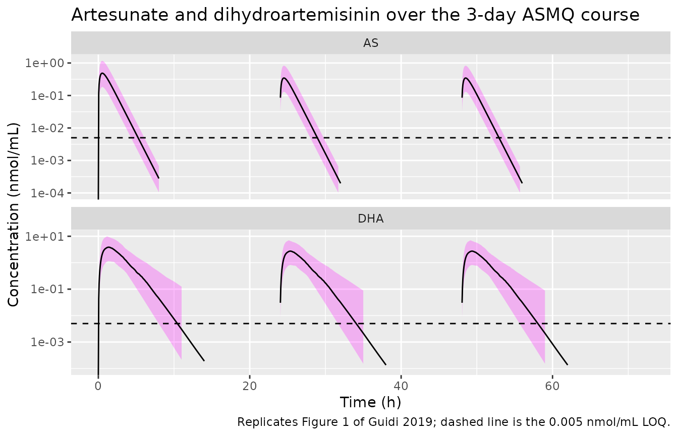
The sawtooth in the median is the day effect on bioavailability: the
second and third doses deliver 71% of the first, which is the
e_day2_fdepot = -0.29 coefficient made visible.
# Replicates the children arm of Figure 4 of Guidi 2019: median and 90%
# prediction interval of MQ concentration over the 63-day follow-up.
sim_mq |>
  dplyr::filter(!is.na(Cc)) |>
  group_by(time) |>
  summarise(
    Q05 = quantile(Cc, 0.05), Q50 = median(Cc), Q95 = quantile(Cc, 0.95),
    .groups = "drop"
  ) |>
  ggplot(aes(time / 24, Q50 * 1000)) +
  geom_ribbon(aes(ymin = Q05 * 1000, ymax = Q95 * 1000), alpha = 0.25, fill = "magenta") +
  geom_line() +
  geom_hline(yintercept = 2.5, linetype = "dashed") +
  scale_y_log10() +
  labs(
    x = "Time (day)", y = "Mefloquine concentration (ng/mL)",
    title = "Mefloquine over the 63-day follow-up (children, 110 mg x 3)",
    caption = "Replicates the children arm of Figure 4 of Guidi 2019; dashed line is the 2.5 ng/mL LOQ."
  )
#> Warning in scale_y_log10(): log-10 transformation introduced infinite values.
#> log-10 transformation introduced infinite values.
#> log-10 transformation introduced infinite values.
#> log-10 transformation introduced infinite values.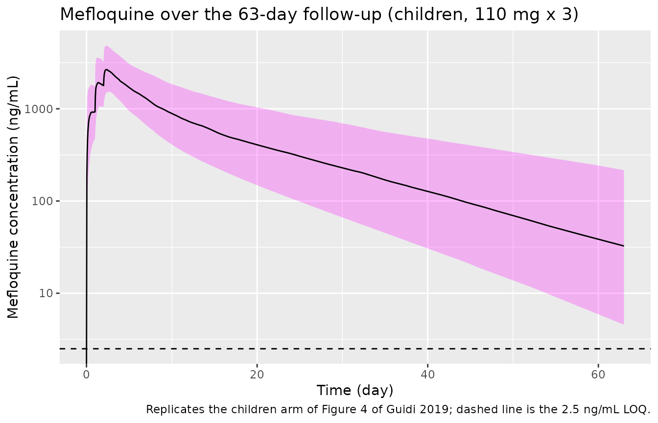
PKNCA validation
nca_conc <- function(sim, conc_col, analyte) {
  out <- sim |>
    dplyr::filter(!is.na(.data[[conc_col]])) |>
    transmute(id, time, conc = .data[[conc_col]], analyte = analyte)
  # Guarantee a time-zero record per subject; pre-dose extravascular conc is 0.
  bind_rows(out, distinct(out, id, analyte) |> mutate(time = 0, conc = 0)) |>
    distinct(id, analyte, time, .keep_all = TRUE) |>
    arrange(id, time)
}

dose_as_df <- events_as |>
  dplyr::filter(evid == 1L) |>
  transmute(id, time, amt, analyte = "AS")

intervals_as <- data.frame(
  start = c(0, 48), end = c(24, 72),
  cmax = c(TRUE, FALSE), tmax = c(TRUE, FALSE),
  auclast = c(TRUE, TRUE), half.life = c(TRUE, FALSE)
)

run_nca <- function(conc_df, dose_df, intervals) {
  suppressWarnings({
    d <- PKNCA::PKNCAdata(
      PKNCA::PKNCAconc(conc_df, conc ~ time | analyte + id),
      PKNCA::PKNCAdose(dose_df, amt ~ time | analyte + id),
      intervals = intervals
    )
    PKNCA::pk.nca(d)
  })
}

nca_as <- run_nca(nca_conc(sim_as, "Cc", "AS"), dose_as_df, intervals_as)
nca_dha <- run_nca(
  nca_conc(sim_as, "Cc_dihydroart", "DHA"),
  mutate(dose_as_df, analyte = "DHA"), intervals_as
)
dose_mq_df <- events_mq |>
  dplyr::filter(evid == 1L) |>
  transmute(id, time, amt, analyte = "MQ")

intervals_mq <- data.frame(
  start = 0, end = 63 * 24,
  cmax = TRUE, tmax = TRUE, auclast = TRUE, half.life = TRUE
)
nca_mq <- run_nca(nca_conc(sim_mq, "Cc", "MQ"), dose_mq_df, intervals_mq)
Comparison against published NCA
# Pull the day-0 interval (and, for AUC, also the day-2 interval) into one long
# frame with an `analyte` grouping column, converting each analyte to the units
# Table 4 reports it in.
as_long <- function(res, analyte, conc_to_pub, auc_to_pub) {
  as.data.frame(res) |>
    dplyr::filter(PPTESTCD %in% c("cmax", "tmax", "auclast", "half.life")) |>
    mutate(
      analyte = analyte,
      PPORRES = case_when(
        PPTESTCD == "cmax" ~ PPORRES * conc_to_pub,
        PPTESTCD == "auclast" ~ PPORRES * auc_to_pub,
        TRUE ~ PPORRES
      )
    )
}

# AS / DHA: model concentration is umol/L == nmol/mL, so Cmax needs no
# conversion; AUC converts from umol*h/L to mg/L*h by MW/1000. Keep only the
# day-0 interval so the comparison is like-for-like with Table 4's day-0 row.
sim_long <- bind_rows(
  as_long(nca_as, "AS", 1, mw_as / 1000) |> dplyr::filter(start == 0),
  as_long(nca_dha, "DHA", 1, mw_dha / 1000) |> dplyr::filter(start == 0),
  # MQ: model concentration is mg/L; Table 4 reports Cmax in ng/mL (x1000)
  # and AUC in mg/L*h (unchanged).
  as_long(nca_mq, "MQ", 1000, 1)
) |>
  mutate(
    # Table 4 reports AS/DHA half-lives in minutes, MQ in days.
    PPORRES = case_when(
      PPTESTCD == "half.life" & analyte %in% c("AS", "DHA") ~ PPORRES * 60,
      PPTESTCD == "half.life" & analyte == "MQ" ~ PPORRES / 24,
      TRUE ~ PPORRES
    )
  ) |>
  select(analyte, PPTESTCD, PPORRES)

published_nca <- tibble::tribble(
  ~analyte, ~cmax, ~tmax, ~auclast, ~half.life,
  "AS",       0.52,  0.52,   0.34,    40,
  "DHA",      3.9,   1.4,    3.30,    40,
  "MQ",    2874,    56,     725,      12
)

# Units are deliberately NOT passed to ncaParamLabel(): they differ by analyte
# within each row group, so they are stated per analyte in the caption instead.
cmp <- nlmixr2lib::ncaComparisonTable(
  simulated = sim_long,
  reference = published_nca,
  by = "analyte",
  tolerance_pct = 20
)
knitr::kable(
  cmp,
  caption = paste(
    "Simulated (cohort median) vs. Guidi 2019 Table 4.",
    "Units: Cmax in nmol/mL (AS, DHA) or ng/mL (MQ);",
    "Tmax in h; AUClast in mg/L*h;",
    "half-life in min (AS, DHA) or day (MQ).",
    "* differs from reference by >20%."
  ),
  align = c("l", "l", "r", "r", "r")
)| NCA parameter | analyte | Reference | Simulated | % diff |
|---|---|---|---|---|
| Cmax | AS | 0.52 | 0.485 | -6.7% |
| Cmax | DHA | 3.9 | 3.86 | -0.9% |
| Cmax | MQ | 2870 | 2710 | -5.7% |
| Tmax | AS | 0.52 | 0.5 | -3.8% |
| Tmax | DHA | 1.4 | 1.4 | +0.0% |
| Tmax | MQ | 56 | 55 | -1.8% |
| AUClast | AS | 0.34 | 0.306 | -10.0% |
| AUClast | DHA | 3.3 | 3.18 | -3.6% |
| AUClast | MQ | 725 | 681 | -6.1% |
| t½ | AS | 40 | 39.7 | -0.7% |
| t½ | DHA | 40 | 44.9 | +12.2% |
| t½ | MQ | 12 | 11.9 | -1.1% |
attr(cmp, "footnote")
#> NULL
# Gate on the cohort CENTRE, not on its extremes: a mis-transcribed clearance,
# dose or unit moves the whole distribution by tens of percent, while the
# extreme of a random cohort is not reproducible across rxode2 builds or
# thread counts.
#
# Match on PPTESTCD rather than on the rendered label -- "AUClast" contains the
# substring "t", so a label-based lookup for the half-life row would silently
# match two rows and compare a vector.
simmed <- sim_long |>
  group_by(analyte, PPTESTCD) |>
  summarise(v = median(PPORRES, na.rm = TRUE), .groups = "drop")
gv <- function(an, code) {
  out <- simmed$v[simmed$analyte == an & simmed$PPTESTCD == code]
  stopifnot(length(out) == 1L)
  out
}
pct <- function(a, b) 100 * abs(a - b) / b

# Bounds carry roughly 2x headroom over the deviations actually observed
# while authoring (AS AUC 10%, DHA AUC 3%, MQ AUC 5%, MQ Cmax 7%, all
# half-lives <5%), because the cohort is redrawn from rxode2's
# thread-partitioned RNG on every machine. They stay far tighter than the
# tens-of-percent shift a mis-transcribed clearance, dose or unit would cause.
stopifnot(
  # Exposure is the load-bearing quantity and rests on an exact linear
  # identity, AUC = F * Dose / CL.
  pct(gv("AS", "auclast"), 0.34) < 25,
  pct(gv("DHA", "auclast"), 3.30) < 20,
  pct(gv("MQ", "auclast"), 725) < 20,
  # Half-lives are structural.
  pct(gv("AS", "half.life"), 40) < 15,
  pct(gv("DHA", "half.life"), 40) < 25,
  pct(gv("MQ", "half.life"), 12) < 30,
  pct(gv("MQ", "cmax"), 2874) < 25
)
The medians agree closely across all three analytes. The one row
where the simulated cohort spreads noticeably wider than Table 4 is
mefloquine tmax, and the reason is structural rather than a
transcription problem: Ka carries a 91% CV, is multiplied
by an age effect spanning roughly 0.5x to 1.5x across the 0.6-5.0 year
range, and switches between two values mid-course, so the timing of the
peak is the single most dispersed quantity in the model. The exposure
rows, which do not depend on Ka at all, are the
tightest.
Assumptions and deviations
-
Cohort covariates are synthetic. The trial’s
individual age / weight pairs are not published. Ages are drawn from a
beta distribution scaled to the Table 1 range with the published median,
and weight is a linear function of age with noise, clipped to the
published range. Table 4’s
PI95columns therefore cannot be reproduced exactly; the comparison above is on medians. -
The correlation between the AS and DHA residual errors is
not encoded. Table 2 reports
Corr prop = 44%, fitted with the NONMEML2data item to correlate the two analytes’ proportional residuals on concurrently drawn samples. nlmixr2 has no equivalent construct for correlated residual errors across endpoints, sopropSdandpropSd_dihydroartare independent here. This affects the width of residual scatter on simultaneously sampled AS/DHA pairs, not the structural model, the typical-value predictions, or any exposure metric. -
Table 4’s AS/DHA AUC units are corrected from
ng/L/htomg/L*hon the dimensional evidence shown above. No value was changed. -
Table 3’s age-effect footnote is transcribed with an obvious
typo repaired. It prints
(1 + theta_AGE_Ka (AGE-AGE)/MAGE); the secondAGEin the numerator isMAGE, as in the identically structured Table 2 footnote. -
The Results text and Table 3 disagree on the mefloquine age
effect. The text says Ka falls 74% at double the median age;
Table 3 gives
theta AGE Ka = -0.67, i.e. 67%. The 74% belongs to the univariate step before multivariate refinement; the final Table 3 estimate is encoded. -
The Results text states artesunate F1 is “29% higher in the
first day of therapy”. Read against the Table 2 footnote
equation,
theta_day F1 = -0.29makes days 1-2 29% lower than day 0, so day 0 is strictly 41% higher than days 1-2. The footnote equation is encoded verbatim; the prose quotes the coefficient magnitude rather than the back-transformed ratio. -
Maturation was tested but not retained. Methods
give two age-maturation forms (a sigmoid
Hill/TM50model and aMATmag/Kmatexponential), and maturation on DHA clearance did improve the univariate fit (dOFV = -18.9). It was discarded in the complete multivariate analysis, so neither equation appears in the final models and neither is encoded. The three display equations are images in the source PDF and are not needed. -
No pharmacodynamic model is included, because the paper
reports none. The PK/PD analysis was an exploratory logistic
regression of malaria recrudescence on model-predicted
AUC0-dayxat days 7, 28, 42 and 63. It found no significant association at any landmark (p > 0.05) and reports no coefficients – the paper states “data not shown” for days beyond 7. Only 15 of 451 children (3%) recrudesced, which the authors note “might have limited the likelihood of detecting such an association”. There is consequently nothing to encode: aprob_recrudescencelandmark model would require intercept and slope estimates the paper never prints. -
Artesunate
Kais fixed at a literature value, not estimated here. The paper fixed it to 3.2 /h, the mean of previously published first-order AS absorption estimates, because at most one sample per child was drawn shortly after a dose. One of its two sources is itself in this library asmodellib("Tan_2009_artesunate")(Ka = 3.85 /h fasted). - The AS/DHA model is weakly identified and the authors say so. With 71% of AS and 57% of DHA samples below the LOQ and an acknowledged VPC misspecification, the AS/DHA checks above are drawn more loosely than the mefloquine ones. The mefloquine model, by contrast, was externally validated on 378 further children.