Naldemedine (Kubota 2018)
Source:vignettes/articles/Kubota_2018_naldemedine.Rmd
Kubota_2018_naldemedine.RmdModel and source
- Citation: Kubota R, Fukumura K, Wajima T. Population Pharmacokinetics and Exposure-Response Relationships of Naldemedine. Pharm Res. 2018;35(11):225. doi:10.1007/s11095-018-2501-7. PMCID: PMC6182381. Final-model parameter estimates and the covariate equations are Table III; the covariate functional forms are Eqs. (1) and (2); baseline covariate distributions are Table II.
- Article: https://doi.org/10.1007/s11095-018-2501-7 (PMCID: PMC6182381, open access)
- Supplementary material (Supplemental Tables S1-S7 and Figures S1-S6): https://doi.org/10.1007/s11095-018-2501-7
Naldemedine is a peripherally acting mu-opioid receptor antagonist for opioid-induced constipation (OIC). Kubota 2018 pooled 8,146 plasma concentrations from 949 subjects across 18 phase 1 to phase 3 studies – healthy volunteers, patients with chronic non-cancer pain and OIC, and cancer patients with OIC – into a single population PK model, then used empirical Bayes steady-state exposures from that model to fit logistic exposure-response models for efficacy and for gastrointestinal safety.
This vignette covers eight models from that one paper:
-
Kubota_2018_naldemedine– the population PK model (two compartments, first-order absorption, absorption lag time). - Seven landmark exposure-response logistic regressions, packaged as
the
Kubota_2018_naldemedine_*family and validated in the Exposure-response models section below, which also closes the loop by feeding PK-simulated steady-state exposures into them.
The seven are split the way the authors fitted them. Kubota 2018 analysed the phase 2b study and the two pooled pivotal phase 3 studies separately, “since the study duration and definition of SBM responders were different”, and fitted each gastrointestinal severity threshold as its own logistic regression. Replicating that structure means seven independent two-parameter fits, not one ordinal model.
mod <- rxode2::rxode(readModelDb("Kubota_2018_naldemedine"))
#> ℹ parameter labels from comments will be replaced by 'label()'
mod
#>  ── rxode2-based free-form 3-cmt ODE model ──────────────────────────────────────
#>  ── Initalization: ──
#> Fixed Effects ($theta):
#>           lcl      e_age_cl     e_crcl_cl e_nonwhite_cl   e_female_cl
#>      2.208274     -0.195000      0.073900      0.870000      0.902000
#>           lvc       e_wt_vc     e_cncp_vc   e_cancer_vc      e_fed_vc
#>      4.329417      1.000000      1.200000      1.270000      1.120000
#>           lka      e_age_ka         ltlag            lq           lvp
#>      1.078410     -1.160000     -1.634756      1.562346      3.732896
#>        propSd
#>      0.257000
#>
#> Omega ($omega):
#>          etalcl   etalvc   etalka    etalq   etalvp
#> etalcl 0.143641 0.000000 0.000000 0.000000 0.000000
#> etalvc 0.000000 0.064009 0.000000 0.000000 0.000000
#> etalka 0.000000 0.000000 2.598544 0.000000 0.000000
#> etalq  0.000000 0.000000 0.000000 0.214369 0.000000
#> etalvp 0.000000 0.000000 0.000000 0.000000 0.131769
#> attr(,"lotriLabels")
#> [1] "Table III IIV CL/F 37.9% CV (95% CI 35.2-40.5), shrinkage 6.6% -> 0.379^2"
#> [2] "Table III IIV Vc/F 25.3% CV (95% CI 20.8-29.2), shrinkage 40.5% -> 0.253^2"
#> [3] "Table III IIV Ka 161.2% CV (95% CI 142.7-177.9), shrinkage 32.6% -> 1.612^2"
#> [4] "Table III IIV Q/F 46.3% CV (95% CI 29.9-58.2), shrinkage 60.6% -> 0.463^2"
#> [5] "Table III IIV Vp/F 36.3% CV (95% CI 30.2-41.6), shrinkage 57.1% -> 0.363^2"
#> attr(,"lotriFix")
#>        etalcl etalvc etalka etalq etalvp
#> etalcl  FALSE  FALSE  FALSE FALSE  FALSE
#> etalvc  FALSE  FALSE  FALSE FALSE  FALSE
#> etalka  FALSE  FALSE  FALSE FALSE  FALSE
#> etalq   FALSE  FALSE  FALSE FALSE  FALSE
#> etalvp  FALSE  FALSE  FALSE FALSE  FALSE
#>
#> States ($state or $stateDf):
#>   Compartment Number Compartment Name
#> 1                  1            depot
#> 2                  2          central
#> 3                  3      peripheral1
#>  ── μ-referencing ($muRefTable): ──
#>   theta    eta level
#> 1   lcl etalcl    id
#> 2   lvc etalvc    id
#> 3   lka etalka    id
#> 4    lq  etalq    id
#> 5   lvp etalvp    id
#>
#>  ── Model (Normalized Syntax): ──
#> function() {
#>     compartmentData <- list(depot = list(analyte = "naldemedine",
#>         units = "mg", specimen = "administration site", verified = TRUE),
#>         central = list(analyte = "naldemedine", units = "mg",
#>             specimen = "plasma", verified = TRUE), peripheral1 = list(analyte = "naldemedine",
#>             units = "mg", specimen = "plasma", verified = TRUE))
#>     covariateData <- list(AGE = list(description = "Age at baseline.",
#>         units = "years", type = "continuous", reference_category = NULL,
#>         notes = "Enters BOTH CL/F and Ka as a median-centred power term, (AGE / 52)^theta, per Kubota 2018 Eq. (1) 'PKP = theta1 x (COV / median of COV)^theta2'. The centring constant 52 years is the cohort median from Table II (mean 51, SD 14, range 18-90). The two exponents have the same sign but very different magnitudes: -0.195 on CL/F (a 90-year-old has CL/F about 10% below the 52-year-old reference) and -1.16 on Ka (the same subject absorbs roughly 1.9-fold more slowly). Age and creatinine clearance are correlated in this cohort (r = -0.45, Supplemental Table S6a), so the two clearance terms are not independently identified; see the vignette.",
#>         source_name = "Age"), CRCL = list(description = "Creatinine clearance at baseline, calculated with the Cockcroft-Gault equation. RAW mL/min, NOT body-surface-area normalised.",
#>         units = "mL/min", type = "continuous", reference_category = NULL,
#>         notes = "Enters CL/F as the median-centred power term (CRCL / 108)^0.0739 per Kubota 2018 Eq. (1). The centring constant 108 mL/min is the cohort median from Table II (mean 109.5, SD 42.4, range 5.8-311.8). IMPORTANT units caveat for reuse: this column is a raw Cockcroft-Gault creatinine clearance in mL/min, whereas the CRCL canonical's primary definition is BSA-normalised mL/min/1.73 m^2. Supplying a BSA-normalised value to this model biases CL/F by (ratio)^0.0739; the exponent is small enough that the error is modest, but it is still an error. The same raw Cockcroft-Gault convention is carried by Delattre_2010_amikacin.R and Jin_2026_colistinSulfate.R. The 95% CI of this exponent includes zero (-0.0133 to 0.161). Kubota 2018 retained the term anyway (Discussion) because a renal-impairment study had shown a real AUC difference; that is a source-stated modelling decision, not an oversight, and it is reproduced here unchanged.",
#>         source_name = "CLcr"), SEXF = list(description = "Female sex indicator.",
#>         units = "(binary)", type = "binary", reference_category = "0 (male)",
#>         notes = "486 of 949 subjects (51.2%) male, 463 (48.8%) female (Table II). Kubota 2018's source indicator is 'Gender = 1 for female, Gender = 0 for male' (Table II footnote), which is exactly the SEXF canonical polarity, so no value transformation is needed. Enters CL/F as the multiplicative power-of-indicator factor 0.902^SEXF per Eq. (2): female CL/F is 9.8% below male.",
#>         source_name = "Gender"), RACE_WHITE = list(description = "White race indicator.",
#>         units = "(binary)", type = "binary", reference_category = "0 (non-White) for the canonical column; note that the SOURCE's reference level is White -- see notes.",
#>         notes = "558 of 949 subjects (58.8%) White, 391 (41.2%) non-White (Table II). POLARITY INVERSION: Kubota 2018's indicator is named 'White' but is coded the other way round -- the Table II footnote states 'White = 1 for non-White, White = 0 for White'. The published factor 0.870 therefore applies to NON-White subjects, whose CL/F is 13% below the White reference. The RACE_WHITE canonical has the opposite polarity, so model() raises the published factor to the power (1 - RACE_WHITE); the estimate itself is carried unchanged and the inversion is visible at the call site. The Results text confirms the footnote independently: the reference population -- the subject at which every indicator is zero, so CL/F is THETA(1) = 9.10 L/h unmodified -- is described as '52-year-old, 76 kg male, white, non-cancer, OIC patients'. That subject is White and carries no race factor, so White = 0 for White. Reading the footnote the other way would move the effect onto the wrong group and invert the direction of a 13% clearance difference. Kubota 2018 tested White/non-White, Japanese/non-Japanese and Hispanic-or-Latino/non-Hispanic-or-non-Latino in SEPARATE models to avoid confounding; only White/non-White was retained.",
#>         source_name = "White"), WT = list(description = "Body weight at baseline.",
#>         units = "kg", type = "continuous", reference_category = NULL,
#>         notes = "Enters Vc/F as the median-centred ratio (WT / 76). The centring constant 76 kg is the cohort median from Table II (mean 79.5, SD 23.4, range 34.4-188.1). Note that Table III writes this term as '* (Body weight/76)' with NO exponent, unlike the age and creatinine-clearance terms which are written as powers -- i.e. the exponent was held at 1 rather than estimated, so ini() carries it as fixed(1).",
#>         source_name = "Body weight"), DIS_HEALTHY = list(description = "Healthy-participant cohort indicator: 1 = healthy subject, 0 = patient (chronic non-cancer pain with OIC, or cancer with OIC).",
#>         units = "(binary)", type = "binary", reference_category = "0 (patient; the complement is the union of the two OIC patient cohorts)",
#>         notes = "Kubota 2018 codes health status with TWO indicator variables over three levels (Table II footnote): 'non-Cancer = 1 and Cancer = 0 for patients with chronic non-cancer pain and OIC, non-Cancer = 0 and Cancer = 1 for cancer patients with OIC, non-Cancer = 0 and Cancer = 0 for healthy subjects'. Healthy subjects are therefore the level at which BOTH source indicators vanish. This model carries the three levels on the two ratified canonicals DIS_HEALTHY and DIS_CANCER rather than minting a new one, and recovers the source's chronic-non-cancer-pain indicator inside model() as dis_cncp_oic = (1 - DIS_HEALTHY) * (1 - DIS_CANCER). Encode a subject as healthy with DIS_HEALTHY = 1, DIS_CANCER = 0; as chronic-non-cancer-pain OIC with both 0; as cancer OIC with DIS_HEALTHY = 0, DIS_CANCER = 1. DIS_HEALTHY = 1 together with DIS_CANCER = 1 is not a state the source data can take and is not defined.",
#>         source_name = "Health status (healthy subjects level)"),
#>         DIS_CANCER = list(description = "Cancer-cohort indicator: 1 = cancer patient with opioid-induced constipation, 0 = healthy subject or patient with chronic non-cancer pain and OIC.",
#>             units = "(binary)", type = "binary", reference_category = "0 (healthy subject or chronic-non-cancer-pain OIC patient)",
#>             notes = "The oncology arm of the pooled analysis: studies 1108V9222 (phase 2b dose finding in cancer patients) and 1331V9236 (phase 3 in Japanese cancer patients). Enters Vc/F as the multiplicative power-of-indicator factor 1.27^DIS_CANCER per Eq. (2): cancer patients have Vc/F 27% above the healthy reference. Note that Kubota 2018's cohort is 'cancer patients with OIC' generally, not specifically the advanced/metastatic solid-tumour population named in the DIS_CANCER register entry's primary description; this is within the entry's paper-defined-complement semantics, which is why its Scope is 'specific'. See DIS_HEALTHY for the full three-level coding scheme.",
#>             source_name = "Health status (cancer level)"), FED = list(description = "Fed-versus-fasted state at the dose record: 1 = fed, 0 = fasted.",
#>             units = "(binary)", type = "binary", reference_category = "0 (fasted)",
#>             notes = "817 of 949 subjects (86.1%) fasted, 132 (13.9%) fed (Table II). The Table II footnote states 'Food = 1 for fed condition, Food = 0 for fasted condition', which matches the FED canonical polarity directly. Enters Vc/F as the multiplicative factor 1.12^FED per Eq. (2). Two source conventions are worth carrying forward when assembling data for this model (Methods): food condition was ASSUMED fasted in the two phase 2b studies (1107V9221, 1108V9222), where food-intake times were not recorded; and in the phase 3 studies it was DEFINED as fasted when naldemedine was given more than 1 h after food.",
#>             source_name = "Food condition"))
#>     covariatesDataExcluded <- list(BMI = list(description = "Body mass index at baseline.",
#>         units = "kg/m^2", type = "continuous", notes = "Tested on CL/F and Vc/F; not retained. Table II: mean 28.1, SD 7.2, median 26.9, range 14.4-58.8."),
#>         ALB = list(description = "Serum albumin at baseline.",
#>             units = "g/dL", type = "continuous", notes = "Tested on CL/F only; not retained. Table II: mean 4.3, SD 0.5, median 4.3, range 2.1-5.4."),
#>         AST = list(description = "Aspartate aminotransferase at baseline.",
#>             units = "U/L", type = "continuous", notes = "Tested on CL/F only; not retained. Table II: mean 22, SD 13, median 19, range 6-223."),
#>         ALT = list(description = "Alanine aminotransferase at baseline.",
#>             units = "U/L", type = "continuous", notes = "Tested on CL/F only; not retained. Table II: mean 22, SD 15, median 18, range 2-212."),
#>         TBILI = list(description = "Total bilirubin at baseline.",
#>             units = "mg/dL", type = "continuous", notes = "Tested on CL/F only; not retained. Table II: mean 0.5, SD 0.3, median 0.4, range 0.04-2.4."),
#>         RACE_JAPANESE = list(description = "Japanese-heritage race indicator.",
#>             units = "(binary)", type = "binary", notes = "249 of 949 (26.2%) Japanese. Tested on CL/F and Vc/F in a SEPARATE model from the White/non-White split, to avoid confounding the race-effect estimate; not retained in the final model."),
#>         RACE_HISPANIC = list(description = "Hispanic or Latino ethnicity indicator.",
#>             units = "(binary)", type = "binary", notes = "96 of 949 (10.1%) Hispanic or Latino. Tested in a SEPARATE model from the other two race/ethnicity splits; not retained."),
#>         AGE_GE65 = list(description = "Categorical age indicator: 1 = 65 years or older, 0 = under 65.",
#>             units = "(binary)", type = "binary", notes = "166 of 949 (17.5%) aged 65 or over. Tested as a categorical alternative to continuous AGE; the continuous power form was retained instead."),
#>         CONMED_PGP_INH = list(description = "Concomitant P-glycoprotein inhibitor indicator.",
#>             units = "(binary)", type = "binary", notes = "Tested on CL/F; not retained. Data from the concomitant-treatment periods of the phase 1 DDI studies (1202V9218 cyclosporine, 1403V921D rifampin, 1502V921E itraconazole/fluconazole) were EXCLUDED from the population PK analysis as worst-case scenarios not clinically relevant to OIC treatment, so this indicator is 1 for only 58 of 949 subjects (6.1%)."),
#>         CONMED_CYP3A_INH = list(description = "Concomitant CYP3A inhibitor indicator (strong or moderate).",
#>             units = "(binary)", type = "binary", notes = "Tested on CL/F; not retained. 14 subjects (1.5%) with a strong and 43 (4.5%) with a moderate inhibitor. See CONMED_PGP_INH for the DDI-period exclusion."),
#>         CONMED_CYP3A_IND = list(description = "Concomitant CYP3A inducer indicator (strong or moderate).",
#>             units = "(binary)", type = "binary", notes = "Tested on CL/F; not retained. 10 subjects (1.1%) with a strong and 6 (0.6%) with a moderate inducer. See CONMED_PGP_INH for the DDI-period exclusion."),
#>         FORM_NALDEMEDINE = list(description = "Formulation category: solution or suspension, phase 1/2 tablet, or phase 3 tablet.",
#>             units = "(categorical)", type = "categorical", notes = "Tested on Ka only; not retained. Table II: solution or suspension 54 (5.7%), phase 1 or 2 tablet 130 (13.7%), phase 3 tablet 765 (80.6%)."))
#>     description <- "Population pharmacokinetic model of naldemedine, a peripherally acting mu-opioid receptor antagonist for opioid-induced constipation (OIC), pooled across 18 phase 1 to phase 3 studies in healthy subjects, patients with chronic non-cancer pain and OIC, and cancer patients with OIC (Kubota 2018, n = 949, 8,146 plasma concentrations). Two-compartment disposition with first-order absorption and an absorption lag time. Apparent oral clearance carries median-centred power effects of age and creatinine clearance plus multiplicative non-White-race and female-sex factors; apparent central volume carries a linear body-weight ratio plus multiplicative health-status (chronic non-cancer pain OIC, cancer OIC) and fed-state factors; the absorption rate constant carries a median-centred power effect of age. The reference subject is a 52-year-old, 76 kg, White, male patient with chronic non-cancer pain and OIC, creatinine clearance 108 mL/min, dosed fasted: CL/F 9.10 L/h, Vc/F 91.1 L, Ka 2.94 1/h, Q/F 4.77 L/h, Vp/F 41.8 L, ALAG 0.195 h. Seven companion landmark exposure-response models in the Kubota_2018_naldemedine_* family relate the steady-state AUC this model produces to the probability of a spontaneous-bowel-movement response and to the probability of gastrointestinal adverse events."
#>     population <- list(species = "human", n_subjects = 949L,
#>         n_studies = 18L, n_observations = "8,146 naldemedine plasma concentrations from 949 subjects. 9,077 samples were drawn from 1,026 subjects; 39 were excluded (14 not measured, 4 with an unidentified sampling or dosing time, 2 detectable before the first dose, 19 unexpected outliers) and 892 below-limit-of- quantification records (402 pre-dose, 490 post-dose) were treated as missing. LLOQ 0.01 ng/mL.",
#>         age_range = "18-90 years (mean 51, SD 14, median 52); 783 (82.5%) under 65 years, 166 (17.5%) 65 or older",
#>         weight_range = "34.4-188.1 kg (mean 79.5, SD 23.4, median 76.0)",
#>         bmi_range = "14.4-58.8 kg/m^2 (mean 28.1, SD 7.2, median 26.9)",
#>         renal_function = "Creatinine clearance (Cockcroft-Gault) 5.8-311.8 mL/min (mean 109.5, SD 42.4, median 108.0); includes a dedicated renal-impairment study (1401V921B, n = 38)",
#>         hepatic_function = "Total bilirubin 0.04-2.4 mg/dL, AST 6-223 U/L, ALT 2-212 U/L, albumin 2.1-5.4 g/dL; includes a dedicated hepatic-impairment study (1402V921C, n = 24)",
#>         sex_female_pct = 48.8, race_ethnicity = c(White = 58.8,
#>             Asian = 26.4, `Black or African American` = 13.5,
#>             `American Indian or Alaska Native` = 0.9, `Native Hawaiian or other Pacific Islander` = 0.2,
#>             Other = 0.1), ethnicity_detail = "Japanese 249 (26.2%); Hispanic or Latino 96 (10.1%)",
#>         disease_state = "Pooled across three populations: healthy subjects (phase 1), patients with chronic non-cancer pain and opioid-induced constipation (phase 2 and phase 3), and cancer patients with opioid-induced constipation (phase 2b study 1108V9222 and phase 3 study 1331V9236). All patient cohorts were on chronic opioid therapy.",
#>         dose_range = "0.01 to 3 mg oral naldemedine, single and multiple dose; the marketed clinical dose is 0.2 mg once daily",
#>         regions = "Global; phase 1 and phase 3 studies in Japan and internationally, with a large Japanese subgroup (26.2%)",
#>         notes = "Analysis dataset pooled from 18 studies spanning phase 1 to phase 3 (Table I). Data from the concomitant-treatment periods of the three phase 1 drug-drug-interaction studies (1202V9218 cyclosporine, 1403V921D rifampin, 1502V921E itraconazole/fluconazole) were excluded because those regimens were designed as worst-case perpetrator exposures and are not clinically relevant to OIC treatment. Fitted in NONMEM 7.3 with FOCE-I; 200-replicate nonparametric bootstrap (98 runs, 49.0%, completed successfully) and a 1000-replicate prediction-corrected VPC were used for evaluation, with 7.4% of observations outside the 90% prediction interval. Kubota 2018 notes that observations above 100 h post-dose tended to exceed predictions; those concentrations are below 1/100 of Cmax and the authors judged the misfit not clinically meaningful.")
#>     reference <- "Kubota R, Fukumura K, Wajima T. Population Pharmacokinetics and Exposure-Response Relationships of Naldemedine. Pharm Res. 2018;35(11):225. doi:10.1007/s11095-018-2501-7. PMCID: PMC6182381. Final-model parameter estimates and the covariate equations are Table III; the covariate functional forms are Eqs. (1) and (2); baseline covariate distributions are Table II."
#>     units <- list(time = "h", dosing = "mg (naldemedine free base; the clinical dose is 0.2 mg once daily)",
#>         concentration = "ng/mL")
#>     vignette <- "Kubota_2018_naldemedine"
#>     ini({
#>         lcl <- 2.2082744135228
#>         label("Apparent oral clearance CL/F (L/h) in the reference subject")
#>         e_age_cl <- -0.195
#>         label("Power exponent of median-centred age (AGE/52) on CL/F (unitless)")
#>         e_crcl_cl <- 0.0739
#>         label("Power exponent of median-centred creatinine clearance (CRCL/108) on CL/F (unitless)")
#>         e_nonwhite_cl <- 0.87
#>         label("Multiplicative factor on CL/F for NON-White race, applied as a power of (1 - RACE_WHITE) (unitless)")
#>         e_female_cl <- 0.902
#>         label("Multiplicative factor on CL/F for female sex, applied as a power of SEXF (unitless)")
#>         lvc <- 4.32941668440158
#>         label("Apparent central volume Vc/F (L) at 76 kg in a HEALTHY subject dosed fasted")
#>         e_wt_vc <- fix(1)
#>         label("Power exponent of median-centred body weight (WT/76) on Vc/F (unitless, held at 1)")
#>         e_cncp_vc <- 1.2
#>         label("Multiplicative factor on Vc/F for chronic-non-cancer-pain OIC patients versus healthy (unitless)")
#>         e_cancer_vc <- 1.27
#>         label("Multiplicative factor on Vc/F for cancer OIC patients versus healthy (unitless)")
#>         e_fed_vc <- 1.12
#>         label("Multiplicative factor on Vc/F for the fed state, applied as a power of FED (unitless)")
#>         lka <- 1.07840958135059
#>         label("First-order absorption rate constant Ka (1/h) at the reference age")
#>         e_age_ka <- -1.16
#>         label("Power exponent of median-centred age (AGE/52) on Ka (unitless)")
#>         ltlag <- -1.63475572041839
#>         label("Absorption lag time ALAG (h)")
#>         lq <- 1.56234630490025
#>         label("Apparent inter-compartmental clearance Q/F (L/h)")
#>         lvp <- 3.73289633953071
#>         label("Apparent peripheral volume Vp/F (L)")
#>         propSd <- c(0, 0.257)
#>         label("Proportional residual error (fraction)")
#>         etalcl ~ 0.143641
#>         label("Table III IIV CL/F 37.9% CV (95% CI 35.2-40.5), shrinkage 6.6% -> 0.379^2")
#>         etalvc ~ 0.064009
#>         label("Table III IIV Vc/F 25.3% CV (95% CI 20.8-29.2), shrinkage 40.5% -> 0.253^2")
#>         etalka ~ 2.598544
#>         label("Table III IIV Ka 161.2% CV (95% CI 142.7-177.9), shrinkage 32.6% -> 1.612^2")
#>         etalq ~ 0.214369
#>         label("Table III IIV Q/F 46.3% CV (95% CI 29.9-58.2), shrinkage 60.6% -> 0.463^2")
#>         etalvp ~ 0.131769
#>         label("Table III IIV Vp/F 36.3% CV (95% CI 30.2-41.6), shrinkage 57.1% -> 0.363^2")
#>     })
#>     model({
#>         dis_cncp_oic <- (1 - DIS_HEALTHY) * (1 - DIS_CANCER)
#>         cl <- exp(lcl + etalcl) * (AGE/52)^e_age_cl * (CRCL/108)^e_crcl_cl *
#>             e_nonwhite_cl^(1 - RACE_WHITE) * e_female_cl^SEXF
#>         vc <- exp(lvc + etalvc) * (WT/76)^e_wt_vc * e_cncp_vc^dis_cncp_oic *
#>             e_cancer_vc^DIS_CANCER * e_fed_vc^FED
#>         ka <- exp(lka + etalka) * (AGE/52)^e_age_ka
#>         q <- exp(lq + etalq)
#>         vp <- exp(lvp + etalvp)
#>         tlag <- exp(ltlag)
#>         kel <- cl/vc
#>         k12 <- q/vc
#>         k21 <- q/vp
#>         d/dt(depot) <- -ka * depot
#>         d/dt(central) <- ka * depot - kel * central - k12 * central +
#>             k21 * peripheral1
#>         d/dt(peripheral1) <- k12 * central - k21 * peripheral1
#>         alag(depot) <- tlag
#>         Cc <- 1000 * central/vc
#>         Cc ~ prop(propSd)
#>     })
#> }
Population
pop <- mod$population
tibble::tibble(
  Field = names(pop),
  Value = vapply(
    pop,
    function(x) paste(if (is.null(names(x))) as.character(x) else paste0(names(x), ": ", x), collapse = "; "),
    character(1)
  )
) |>
knitr::kable(caption = "Population metadata (Kubota 2018 Tables I and II).")| Field | Value |
|---|---|
| species | human |
| n_subjects | 949 |
| n_studies | 18 |
| n_observations | 8,146 naldemedine plasma concentrations from 949 subjects. 9,077 samples were drawn from 1,026 subjects; 39 were excluded (14 not measured, 4 with an unidentified sampling or dosing time, 2 detectable before the first dose, 19 unexpected outliers) and 892 below-limit-of- quantification records (402 pre-dose, 490 post-dose) were treated as missing. LLOQ 0.01 ng/mL. |
| age_range | 18-90 years (mean 51, SD 14, median 52); 783 (82.5%) under 65 years, 166 (17.5%) 65 or older |
| weight_range | 34.4-188.1 kg (mean 79.5, SD 23.4, median 76.0) |
| bmi_range | 14.4-58.8 kg/m^2 (mean 28.1, SD 7.2, median 26.9) |
| renal_function | Creatinine clearance (Cockcroft-Gault) 5.8-311.8 mL/min (mean 109.5, SD 42.4, median 108.0); includes a dedicated renal-impairment study (1401V921B, n = 38) |
| hepatic_function | Total bilirubin 0.04-2.4 mg/dL, AST 6-223 U/L, ALT 2-212 U/L, albumin 2.1-5.4 g/dL; includes a dedicated hepatic-impairment study (1402V921C, n = 24) |
| sex_female_pct | 48.8 |
| race_ethnicity | White: 58.8; Asian: 26.4; Black or African American: 13.5; American Indian or Alaska Native: 0.9; Native Hawaiian or other Pacific Islander: 0.2; Other: 0.1 |
| ethnicity_detail | Japanese 249 (26.2%); Hispanic or Latino 96 (10.1%) |
| disease_state | Pooled across three populations: healthy subjects (phase 1), patients with chronic non-cancer pain and opioid-induced constipation (phase 2 and phase 3), and cancer patients with opioid-induced constipation (phase 2b study 1108V9222 and phase 3 study 1331V9236). All patient cohorts were on chronic opioid therapy. |
| dose_range | 0.01 to 3 mg oral naldemedine, single and multiple dose; the marketed clinical dose is 0.2 mg once daily |
| regions | Global; phase 1 and phase 3 studies in Japan and internationally, with a large Japanese subgroup (26.2%) |
| notes | Analysis dataset pooled from 18 studies spanning phase 1 to phase 3 (Table I). Data from the concomitant-treatment periods of the three phase 1 drug-drug-interaction studies (1202V9218 cyclosporine, 1403V921D rifampin, 1502V921E itraconazole/fluconazole) were excluded because those regimens were designed as worst-case perpetrator exposures and are not clinically relevant to OIC treatment. Fitted in NONMEM 7.3 with FOCE-I; 200-replicate nonparametric bootstrap (98 runs, 49.0%, completed successfully) and a 1000-replicate prediction-corrected VPC were used for evaluation, with 7.4% of observations outside the 90% prediction interval. Kubota 2018 notes that observations above 100 h post-dose tended to exceed predictions; those concentrations are below 1/100 of Cmax and the authors judged the misfit not clinically meaningful. |
The reference subject against which every covariate effect is centred
is, in the paper’s own words, “52-year-old, 76 kg male, white,
non-cancer, OIC patients with CLcr of 108 ml/min, administed under
fasted condintion”. Note that this is a patient with chronic
non-cancer pain, not a healthy volunteer – which is why the
reference Vc/F of 91.1 L is THETA(6) * 1.20, not
THETA(6).
Source trace
Every structural value in the model file, with its source location.
tibble::tribble(
  ~Quantity,                  ~`Model parameter`, ~Value,     ~`Source location`,
  "CL/F, reference",          "lcl",              "9.10 L/h", "Table III THETA(1)",
  "Age exponent on CL/F",     "e_age_cl",         "-0.195",   "Table III THETA(2); Eq. (1)",
  "CLcr exponent on CL/F",    "e_crcl_cl",        "0.0739",   "Table III THETA(3); Eq. (1)",
  "Non-White factor on CL/F", "e_nonwhite_cl",    "0.870",    "Table III THETA(4); Eq. (2)",
  "Female factor on CL/F",    "e_female_cl",      "0.902",    "Table III THETA(5); Eq. (2)",
  "Vc/F, healthy at 76 kg",   "lvc",              "75.9 L",   "Table III THETA(6)",
  "Weight exponent on Vc/F",  "e_wt_vc",          "1 (fixed)", "Table III writes '* (Body weight/76)' with no exponent",
  "Non-cancer factor Vc/F",   "e_cncp_vc",        "1.20",     "Table III THETA(7); Eq. (2)",
  "Cancer factor on Vc/F",    "e_cancer_vc",      "1.27",     "Table III THETA(8); Eq. (2)",
  "Fed factor on Vc/F",       "e_fed_vc",         "1.12",     "Table III THETA(9); Eq. (2)",
  "Ka, reference",            "lka",              "2.94 1/h", "Table III THETA(10)",
  "Age exponent on Ka",       "e_age_ka",         "-1.16",    "Table III THETA(11); Eq. (1)",
  "Q/F",                      "lq",               "4.77 L/h", "Table III",
  "Vp/F",                     "lvp",              "41.8 L",   "Table III",
  "ALAG",                     "ltlag",            "0.195 h",  "Table III",
  "IIV CL/F",                 "etalcl",           "37.9% CV", "Table III",
  "IIV Vc/F",                 "etalvc",           "25.3% CV", "Table III",
  "IIV Ka",                   "etalka",           "161.2% CV", "Table III",
  "IIV Q/F",                  "etalq",            "46.3% CV", "Table III",
  "IIV Vp/F",                 "etalvp",           "36.3% CV", "Table III",
  "Proportional residual",    "propSd",           "25.7% CV", "Table III, intra-individual variability"
) |>
knitr::kable(caption = "Source trace for the population PK model.")| Quantity | Model parameter | Value | Source location |
|---|---|---|---|
| CL/F, reference | lcl | 9.10 L/h | Table III THETA(1) |
| Age exponent on CL/F | e_age_cl | -0.195 | Table III THETA(2); Eq. (1) |
| CLcr exponent on CL/F | e_crcl_cl | 0.0739 | Table III THETA(3); Eq. (1) |
| Non-White factor on CL/F | e_nonwhite_cl | 0.870 | Table III THETA(4); Eq. (2) |
| Female factor on CL/F | e_female_cl | 0.902 | Table III THETA(5); Eq. (2) |
| Vc/F, healthy at 76 kg | lvc | 75.9 L | Table III THETA(6) |
| Weight exponent on Vc/F | e_wt_vc | 1 (fixed) | Table III writes ‘* (Body weight/76)’ with no exponent |
| Non-cancer factor Vc/F | e_cncp_vc | 1.20 | Table III THETA(7); Eq. (2) |
| Cancer factor on Vc/F | e_cancer_vc | 1.27 | Table III THETA(8); Eq. (2) |
| Fed factor on Vc/F | e_fed_vc | 1.12 | Table III THETA(9); Eq. (2) |
| Ka, reference | lka | 2.94 1/h | Table III THETA(10) |
| Age exponent on Ka | e_age_ka | -1.16 | Table III THETA(11); Eq. (1) |
| Q/F | lq | 4.77 L/h | Table III |
| Vp/F | lvp | 41.8 L | Table III |
| ALAG | ltlag | 0.195 h | Table III |
| IIV CL/F | etalcl | 37.9% CV | Table III |
| IIV Vc/F | etalvc | 25.3% CV | Table III |
| IIV Ka | etalka | 161.2% CV | Table III |
| IIV Q/F | etalq | 46.3% CV | Table III |
| IIV Vp/F | etalvp | 36.3% CV | Table III |
| Proportional residual | propSd | 25.7% CV | Table III, intra-individual variability |
The exposure-response coefficients are traced in their own section below.
Which CV convention does Table III use?
Table III reports inter-individual variability as a percent CV
without saying whether it is the approximate CV
(100 * sqrt(omega^2)) or the exact log-normal CV
(100 * sqrt(exp(omega^2) - 1)). The two differ enormously
for Ka, whose CV is 161.2%: omega^2 is 2.599 under the
first reading and 1.281 under the second.
The printed 95% confidence intervals settle it. NONMEM’s covariance step produces an interval that is symmetric on the estimated variance, so back-transforming the printed CV endpoints with the correct formula must restore that symmetry. The test below does exactly that, and is decisive on the two widest intervals – which are also the two where the readings diverge most.
cvtab <- tibble::tribble(
  ~Parameter, ~CV,    ~Lower, ~Upper,
  "CL/F",      37.9,   35.2,   40.5,
  "Vc/F",      25.3,   20.8,   29.2,
  "Ka",       161.2,  142.7,  177.9,
  "Q/F",       46.3,   29.9,   58.2,
  "Vp/F",      36.3,   30.2,   41.6
) |>
  dplyr::mutate(
    # Half-width ratio (upper / lower) of the back-transformed interval.
    # A value near 1 means the transform restored the symmetry NONMEM produced.
    approx_ratio = ((Upper / 100)^2 - (CV / 100)^2) / ((CV / 100)^2 - (Lower / 100)^2),
    exact_ratio = (log(1 + (Upper / 100)^2) - log(1 + (CV / 100)^2)) /
      (log(1 + (CV / 100)^2) - log(1 + (Lower / 100)^2)),
    `omega^2 used` = (CV / 100)^2
  )

cvtab |>
  dplyr::select(
    Parameter, `CV%` = CV, Lower, Upper,
    `Symmetry, omega2=(CV)^2` = approx_ratio,
    `Symmetry, omega2=log(1+CV2)` = exact_ratio,
    `omega^2 used`
  ) |>
  dplyr::mutate(dplyr::across(where(is.numeric), \(x) round(x, 4))) |>
knitr::kable(caption = "Back-transformed CI symmetry under the two readings of Table III's CV% column. A ratio near 1 is the correct reading.")| Parameter | CV% | Lower | Upper | Symmetry, omega2=(CV)^2 | Symmetry, omega2=log(1+CV2) | omega^2 used |
|---|---|---|---|---|---|---|
| CL/F | 37.9 | 35.2 | 40.5 | 1.0328 | 1.0148 | 0.1436 |
| Vc/F | 25.3 | 20.8 | 29.2 | 1.0246 | 1.0046 | 0.0640 |
| Ka | 161.2 | 142.7 | 177.9 | 1.0073 | 0.8603 | 2.5985 |
| Q/F | 46.3 | 29.9 | 58.2 | 0.9951 | 0.8977 | 0.2144 |
| Vp/F | 36.3 | 30.2 | 41.6 | 1.0178 | 0.9816 | 0.1318 |
# Ka and Q/F have by far the widest intervals and therefore the most
# discriminating power; the other three are near-linear under both transforms
# and cannot decide. These bounds are deterministic arithmetic on printed
# numbers -- no simulation is involved -- so they are gated tightly.
disc <- cvtab |> dplyr::filter(Parameter %in% c("Ka", "Q/F"))
stopifnot(
  nrow(disc) == 2L,
  max(abs(disc$approx_ratio - 1)) < 0.02,
  min(abs(disc$exact_ratio - 1)) > 0.08
)

# And the values actually packaged in the model file match that reading.
packaged <- mod$iniDf$est[match(c("etalcl", "etalvc", "etalka", "etalq", "etalvp"), mod$iniDf$name)]
stopifnot(max(abs(packaged - cvtab$`omega^2 used`)) < 1e-6)
The approximate reading is symmetric to within 0.7% on Ka and 0.5% on
Q/F; the exact log-normal reading is 14% and 10% out. Table III’s CV%
column is 100 * sqrt(omega^2), and that is what the model
file carries.
Structural checks (typical value, no random effects)
The reference subject reproduces the published anchors
ref_cov <- data.frame(
  AGE = 52, WT = 76, CRCL = 108, SEXF = 0, RACE_WHITE = 1,
  DIS_HEALTHY = 0, DIS_CANCER = 0, FED = 0
)

solve_typical <- function(ui, cov, ev) {
  ev <- as.data.frame(ev)
  ev <- cbind(ev, cov[rep(1L, nrow(ev)), , drop = FALSE])
  rxode2::rxSolve(rxode2::zeroRe(ui), ev, returnType = "data.frame")
}

ev_single <- rxode2::et(amt = 0.2, cmt = "depot") |>
  rxode2::et(seq(0, 72, by = 0.01), cmt = "central")

ref <- solve_typical(mod, ref_cov, ev_single)
#> ℹ omega/sigma items treated as zero: 'etalcl', 'etalvc', 'etalka', 'etalq', 'etalvp'
ref <- ref[!is.na(ref$Cc), ]

anchors <- tibble::tribble(
  ~Quantity,   ~Published, ~Simulated,
  "CL/F (L/h)",    9.10,   ref$cl[1],
  "Vc/F (L)",     91.1,    ref$vc[1],
  "Ka (1/h)",      2.94,   ref$ka[1],
  "Q/F (L/h)",     4.77,   ref$q[1],
  "Vp/F (L)",     41.8,    ref$vp[1],
  "ALAG (h)",      0.195,  ref$tlag[1]
) |>
  dplyr::mutate(`% difference` = round(100 * (Simulated - Published) / Published, 4))

anchors |>
  dplyr::mutate(Simulated = round(Simulated, 4)) |>
knitr::kable(caption = "Reference-subject parameters against Kubota 2018 Results. Vc/F 91.1 L is THETA(6) x 1.20, because the reference subject is a chronic-non-cancer-pain patient, not a healthy volunteer.")| Quantity | Published | Simulated | % difference |
|---|---|---|---|
| CL/F (L/h) | 9.100 | 9.100 | 0.000 |
| Vc/F (L) | 91.100 | 91.080 | -0.022 |
| Ka (1/h) | 2.940 | 2.940 | 0.000 |
| Q/F (L/h) | 4.770 | 4.770 | 0.000 |
| Vp/F (L) | 41.800 | 41.800 | 0.000 |
| ALAG (h) | 0.195 | 0.195 | 0.000 |
The ODE system really is two-compartment
A cl / vc pair in model() can
make rxode2 substitute an analytic solution for the explicit
d/dt block. That substitution is only harmless when the
parameter set is complete: with q and vp
missing, a two-compartment model silently collapses to one compartment
and every AUC-based check still passes. This model does supply
q and vp, so both readings should coincide –
but “should” is not a check. The gate below compares the solve against
an independently written closed-form two-compartment
first-order-absorption solution with lag.
p <- ref[1, c("cl", "vc", "ka", "q", "vp", "tlag")]
kel <- p$cl / p$vc
k12 <- p$q / p$vc
k21 <- p$q / p$vp
bsum <- kel + k12 + k21
disc2 <- sqrt(bsum^2 - 4 * kel * k21)
alpha <- (bsum + disc2) / 2
beta <- (bsum - disc2) / 2

tt <- pmax(ref$time - p$tlag, 0)
cf <- 1000 * 0.2 * p$ka / p$vc * (
  (k21 - p$ka) / ((alpha - p$ka) * (beta - p$ka)) * exp(-p$ka * tt) +
    (k21 - alpha) / ((p$ka - alpha) * (beta - alpha)) * exp(-alpha * tt) +
    (k21 - beta) / ((p$ka - beta) * (alpha - beta)) * exp(-beta * tt)
)
cf[ref$time < p$tlag] <- 0

keep <- cf > 1e-6
rel_err <- max(abs(ref$Cc[keep] - cf[keep]) / cf[keep])

cat(sprintf(
  "alpha = %.4f 1/h, beta = %.4f 1/h (t1/2 = %.2f h); max relative error = %.2e over %d points\n",
  alpha, beta, log(2) / beta, rel_err, sum(keep)
))
#> alpha = 0.2128 1/h, beta = 0.0536 1/h (t1/2 = 12.94 h); max relative error = 2.47e-06 over 7181 points

stopifnot(
  # Numerical solver agreement, not a cohort statistic: tight.
  rel_err < 1e-4,
  # Two DISTINCT disposition phases -- a collapsed one-compartment model would
  # not produce them.
  alpha > 3 * beta,
  # The lag is honoured.
  all(ref$Cc[ref$time < p$tlag] == 0)
)
The paper’s own covariate-extremes calculation
This is the single most informative check in the paper. Kubota 2018 states that if age (18-90 years), CLcr (5.8-311 mL/min), race and gender independently took their most extreme values, “the population predicted CL/F would range from 5.17 to 12.1 L/h, which would decrease the population predicted AUCss by 25% or would increase by 76%”.
Reproducing those four numbers is an end-to-end check on the continuous covariate terms: both centring constants (52 years, 108 mL/min), both exponents, and the magnitude of the two categorical factors all have to be right for the bounds to land. Note what it does not test: because the paper lets each covariate “independently take extreme values”, the optimum is free to pick either level of a binary covariate, so the extremes are the same whichever way the race and gender indicators are coded. The polarity question is settled by the reference-subject anchor above, not here (see Assumptions and deviations).
cl_typ <- function(age, crcl, race_white, sexf) {
  ini <- mod$iniDf$est[match(
    c("lcl", "e_age_cl", "e_crcl_cl", "e_nonwhite_cl", "e_female_cl"),
    mod$iniDf$name
  )]
  exp(ini[1]) * (age / 52)^ini[2] * (crcl / 108)^ini[3] *
    ini[4]^(1 - race_white) * ini[5]^sexf
}

# Highest CL/F: youngest, best renal function, White, male.
cl_hi <- cl_typ(age = 18, crcl = 311.8, race_white = 1, sexf = 0)
# Lowest CL/F: oldest, worst renal function, non-White, female.
cl_lo <- cl_typ(age = 90, crcl = 5.8, race_white = 0, sexf = 1)

extremes <- tibble::tribble(
  ~Quantity,                  ~Published, ~Reproduced,
  "Highest CL/F (L/h)",          12.1,    cl_hi,
  "Lowest CL/F (L/h)",            5.17,   cl_lo,
  "AUCss change, highest CL/F (%)", -25,  100 * (9.10 / cl_hi - 1),
  "AUCss change, lowest CL/F (%)",   76,  100 * (9.10 / cl_lo - 1)
) |>
  dplyr::mutate(`Absolute difference` = abs(Reproduced - Published))

extremes |>
  dplyr::mutate(Reproduced = round(Reproduced, 3), `Absolute difference` = round(`Absolute difference`, 3)) |>
knitr::kable(caption = "Kubota 2018 Results, covariate-extremes paragraph, reproduced from the packaged parameters.")| Quantity | Published | Reproduced | Absolute difference |
|---|---|---|---|
| Highest CL/F (L/h) | 12.10 | 12.104 | 0.004 |
| Lowest CL/F (L/h) | 5.17 | 5.170 | 0.000 |
| AUCss change, highest CL/F (%) | -25.00 | -24.815 | 0.185 |
| AUCss change, lowest CL/F (%) | 76.00 | 76.029 | 0.029 |
# Deterministic arithmetic on printed values. The published CL/F bounds carry 3
# significant figures and the AUCss percentages are printed as integers, so the
# tolerances below are the paper's own rounding, not slack.
stopifnot(
  abs(cl_hi - 12.1) < 0.01,
  abs(cl_lo - 5.17) < 0.01,
  abs(100 * (9.10 / cl_hi - 1) - (-25)) < 0.5,
  abs(100 * (9.10 / cl_lo - 1) - 76) < 0.5
)
Steady-state exposure identity
Naldemedine PK is linear, so at steady state on a once-daily regimen
AUCtau = Dose / (CL/F) exactly. Kubota 2018 reports 21.98
ng*h/mL for the reference subject at 0.2 mg once daily, and derived
every individual AUCss used in the exposure-response analysis the same
way.
ev_ss <- rxode2::et(amt = 0.2, cmt = "depot", ii = 24, addl = 14) |>
  rxode2::et(seq(0, 24 * 15, by = 0.05), cmt = "central")

ss <- solve_typical(mod, ref_cov, ev_ss)
#> ℹ omega/sigma items treated as zero: 'etalcl', 'etalvc', 'etalka', 'etalq', 'etalvp'
ss <- ss[!is.na(ss$Cc), ]
last <- ss[ss$time >= 24 * 14, ]
auc_tau <- sum(diff(last$time) * (utils::head(last$Cc, -1) + utils::tail(last$Cc, -1)) / 2)
auc_id <- 1000 * 0.2 / ss$cl[1]

cat(sprintf(
  "AUCtau (trapezoid over the 15th interval) = %.4f ng*h/mL\nDose / (CL/F)                           = %.4f ng*h/mL\nKubota 2018 Results                     = 21.98 ng*h/mL\n",
  auc_tau, auc_id
))
#> AUCtau (trapezoid over the 15th interval) = 21.9774 ng*h/mL
#> Dose / (CL/F)                           = 21.9780 ng*h/mL
#> Kubota 2018 Results                     = 21.98 ng*h/mL

stopifnot(
  # Mass-balance identity: numerical, so tight.
  abs(auc_tau / auc_id - 1) < 0.002,
  # Against the published typical value (printed to 4 significant figures).
  abs(auc_tau - 21.98) < 0.05
)
Virtual cohort
The cohort replicates the design of the phase 2b dose-finding study 1107V9221 – patients with chronic non-cancer pain and OIC, dosed once daily under fasted conditions at 0.1, 0.2 and 0.4 mg – because that is the arm structure Supplemental Table S4 reports observed steady-state exposures for. Covariates are drawn from the pooled Table II marginal distributions and truncated to the observed ranges.
set.seed(20181002)
rxode2::rxSetSeed(20181002)

n_per_arm <- 120L
doses <- c(0.1, 0.2, 0.4)

rtrunc <- function(n, mean, sd, lo, hi) pmin(pmax(stats::rnorm(n, mean, sd), lo), hi)

cohort <- tidyr::expand_grid(
  dose = doses,
  k = seq_len(n_per_arm)
) |>
  dplyr::mutate(
    id = dplyr::row_number(),
    arm = paste0(format(dose, trim = TRUE), " mg"),
    # Table II continuous covariates: mean, SD and observed range.
    AGE = rtrunc(dplyr::n(), 51, 14, 18, 90),
    WT = rtrunc(dplyr::n(), 79.5, 23.4, 34.4, 188.1),
    CRCL = rtrunc(dplyr::n(), 109.5, 42.4, 5.8, 311.8),
    # Table II categorical covariates.
    SEXF = stats::rbinom(dplyr::n(), 1L, 0.488),
    RACE_WHITE = stats::rbinom(dplyr::n(), 1L, 0.588),
    # Study 1107V9221 enrolled patients with chronic non-cancer pain and OIC,
    # dosed fasted: neither the healthy nor the cancer indicator is set.
    DIS_HEALTHY = 0,
    DIS_CANCER = 0,
    FED = 0
  ) |>
  dplyr::select(-k)

stopifnot(nrow(cohort) == n_per_arm * length(doses), max(table(cohort$arm)) <= 200L)

cohort |>
  dplyr::group_by(arm) |>
  dplyr::summarise(
    n = dplyr::n(),
    `Age (median)` = round(stats::median(AGE), 1),
    `Weight (median)` = round(stats::median(WT), 1),
    `CLcr (median)` = round(stats::median(CRCL), 1),
    `Female %` = round(100 * mean(SEXF), 1),
    `White %` = round(100 * mean(RACE_WHITE), 1),
    .groups = "drop"
  ) |>
knitr::kable(caption = "Virtual cohort, drawn from the Kubota 2018 Table II marginal covariate distributions.")| arm | n | Age (median) | Weight (median) | CLcr (median) | Female % | White % |
|---|---|---|---|---|---|---|
| 0.1 mg | 120 | 49.6 | 80.1 | 115.4 | 48.3 | 59.2 |
| 0.2 mg | 120 | 49.8 | 79.7 | 111.8 | 45.8 | 60.8 |
| 0.4 mg | 120 | 50.0 | 84.4 | 109.4 | 55.0 | 55.8 |
Simulation
Fifteen once-daily doses to reach steady state, then a dense observation grid over the final dosing interval.
dose_rows <- cohort |>
  dplyr::transmute(
    id, arm, AGE, WT, CRCL, SEXF, RACE_WHITE, DIS_HEALTHY, DIS_CANCER, FED,
    time = 0, amt = dose, evid = 1L, cmt = "depot", ii = 24, addl = 14L
  )

obs_rows <- cohort |>
  dplyr::select(id, arm, AGE, WT, CRCL, SEXF, RACE_WHITE, DIS_HEALTHY, DIS_CANCER, FED) |>
  tidyr::crossing(time = 24 * 14 + seq(0, 24, by = 0.25)) |>
  dplyr::mutate(
    amt = NA_real_, evid = 0L,
    # The ODE STATE name, never the observable name "Cc" -- referencing an
    # algebraic observable as a compartment renumbers the compartment slots.
    cmt = "central",
    ii = 0, addl = 0L
  )

events <- dplyr::bind_rows(dose_rows, obs_rows) |>
  dplyr::arrange(id, time, dplyr::desc(evid)) |>
  as.data.frame()

sim <- rxode2::rxSolve(mod, events, returnType = "data.frame")
if (is.null(sim$id)) sim$id <- 1L

# rxSolve drops character columns such as `arm`, so join the cohort labels back
# by id. The join must be total -- a partial match would silently shrink the
# cohort and every downstream summary with it.
sim <- sim |>
  dplyr::mutate(id = as.integer(as.character(id))) |>
  dplyr::left_join(dplyr::select(cohort, id, arm, dose), by = "id") |>
  dplyr::filter(!is.na(Cc)) |>
  dplyr::mutate(tad = time - 24 * 14)

stopifnot(
  nrow(sim) > 0L, all(sim$Cc >= 0), !anyNA(sim$Cc),
  !anyNA(sim$arm),
  dplyr::n_distinct(sim$id) == nrow(cohort)
)
Steady-state concentration-time profiles
sim |>
  dplyr::group_by(arm, tad) |>
  dplyr::summarise(
    lo = stats::quantile(Cc, 0.05),
    md = stats::median(Cc),
    hi = stats::quantile(Cc, 0.95),
    .groups = "drop"
  ) |>
  ggplot2::ggplot(ggplot2::aes(tad, md, colour = arm, fill = arm)) +
  ggplot2::geom_ribbon(ggplot2::aes(ymin = lo, ymax = hi), alpha = 0.15, colour = NA) +
  ggplot2::geom_line(linewidth = 0.8) +
  ggplot2::scale_y_log10() +
  ggplot2::labs(
    x = "Time after dose (h)", y = "Naldemedine concentration (ng/mL)",
    colour = "Dose", fill = "Dose"
  ) +
  ggplot2::theme_bw()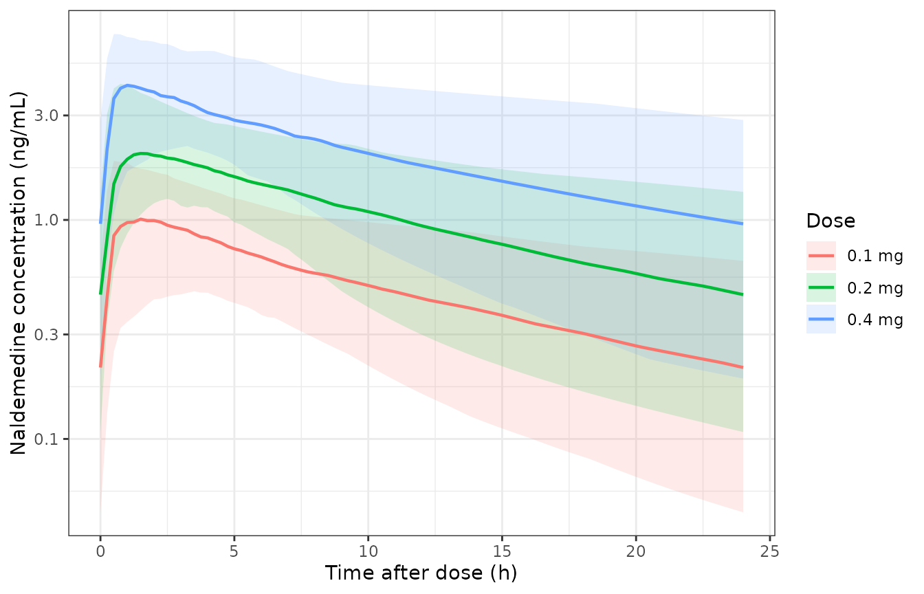
Simulated steady-state naldemedine profiles over the final 24 h dosing interval at 0.1, 0.2 and 0.4 mg once daily (median and 5th-95th percentile band). Compare with the observed spread in Kubota 2018 Figure 1b and the prediction-corrected VPC in Figure 2.
The profiles are dose-proportional, as the linear model requires: the bands at 0.1, 0.2 and 0.4 mg are vertical translations of one another on the log scale.
PKNCA validation
Non-compartmental analysis over the steady-state interval, grouped by dose arm so each arm can be compared against its own Supplemental Table S4 row.
conc_data <- sim |>
  dplyr::filter(!is.na(Cc)) |>
  dplyr::select(id, arm, time, Cc)

# Defensive time-zero anchor: PKNCA warns on every subject if the interval
# starts before the first measurement. The grid above already contains
# tad = 0, so this is a no-op here, kept so the block stays correct if the
# grid is ever coarsened.
conc_data <- conc_data |>
  dplyr::bind_rows(
    sim |>
      dplyr::filter(tad == 0) |>
      dplyr::select(id, arm, time, Cc)
  ) |>
  dplyr::distinct(id, arm, time, .keep_all = TRUE) |>
  dplyr::arrange(id, time)

dose_data <- cohort |>
  dplyr::transmute(id, arm, time = 24 * 14, dose = dose)

o_conc <- PKNCA::PKNCAconc(conc_data, Cc ~ time | id / arm)
# PKNCAdose does not accept slash (nested) grouping, only PKNCAconc does.
o_dose <- PKNCA::PKNCAdose(dose_data, dose ~ time | id + arm)

intervals <- data.frame(
  start = 24 * 14, end = 24 * 15,
  auclast = TRUE, cmax = TRUE, cmin = TRUE, tmax = TRUE
)

o_nca <- PKNCA::pk.nca(PKNCA::PKNCAdata(o_conc, o_dose, intervals = intervals))

nca_res <- as.data.frame(o_nca) |>
  dplyr::filter(PPTESTCD %in% c("auclast", "cmax", "cmin", "tmax"))

stopifnot(nrow(nca_res) > 0L, !anyNA(nca_res$PPORRES))
nca_summary <- nca_res |>
  dplyr::group_by(arm, PPTESTCD) |>
  dplyr::summarise(
    gm = exp(mean(log(pmax(PPORRES, 1e-12)))),
    md = stats::median(PPORRES),
    cv = 100 * sqrt(exp(stats::var(log(pmax(PPORRES, 1e-12)))) - 1),
    .groups = "drop"
  )

nca_summary |>
  dplyr::mutate(
    Parameter = dplyr::recode(
      PPTESTCD,
      auclast = "AUCss (ng*h/mL)",
      cmax = "Cmax,ss (ng/mL)",
      cmin = "Cmin,ss (ng/mL)",
      tmax = "Tmax (h)"
    ),
    `Geometric mean` = round(gm, 3),
    Median = round(md, 3),
    `CV%` = round(cv, 1)
  ) |>
  dplyr::select(Arm = arm, Parameter, `Geometric mean`, Median, `CV%`) |>
knitr::kable(caption = "Simulated steady-state exposure by dose arm.")| Arm | Parameter | Geometric mean | Median | CV% |
|---|---|---|---|---|
| 0.1 mg | AUCss (ng*h/mL) | 11.615 | 11.781 | 44.9 |
| 0.1 mg | Cmax,ss (ng/mL) | 1.080 | 1.103 | 40.0 |
| 0.1 mg | Cmin,ss (ng/mL) | 0.180 | 0.212 | 117.1 |
| 0.1 mg | Tmax (h) | 1.225 | 1.250 | 98.6 |
| 0.2 mg | AUCss (ng*h/mL) | 26.045 | 25.195 | 41.0 |
| 0.2 mg | Cmax,ss (ng/mL) | 2.244 | 2.129 | 38.4 |
| 0.2 mg | Cmin,ss (ng/mL) | 0.448 | 0.456 | 94.1 |
| 0.2 mg | Tmax (h) | 1.458 | 1.500 | 96.0 |
| 0.4 mg | AUCss (ng*h/mL) | 48.980 | 47.657 | 46.3 |
| 0.4 mg | Cmax,ss (ng/mL) | 4.323 | 4.334 | 36.7 |
| 0.4 mg | Cmin,ss (ng/mL) | 0.824 | 0.960 | 109.8 |
| 0.4 mg | Tmax (h) | 1.247 | 1.000 | 93.1 |
The NCA AUC recovers Dose / (CL/F) per subject
The strongest available internal check: because the model is linear,
each subject’s steady-state AUCtau must equal that subject’s
Dose / (CL/F). This is a per-subject identity, so it tests
the covariate model, the dosing path and the solver all at once, and it
cannot be satisfied by a mis-specified compartment structure that
happens to have the right clearance.
subj_cl <- sim |>
  dplyr::group_by(id, arm) |>
  dplyr::summarise(cl = dplyr::first(cl), .groups = "drop")

auc_check <- nca_res |>
  dplyr::filter(PPTESTCD == "auclast") |>
  dplyr::select(id, arm, auc = PPORRES) |>
  dplyr::inner_join(subj_cl, by = c("id", "arm")) |>
  dplyr::inner_join(dplyr::select(cohort, id, dose), by = "id") |>
  dplyr::mutate(
    expected = 1000 * dose / cl,
    pct_diff = 100 * (auc - expected) / expected
  )

stopifnot(nrow(auc_check) == nrow(cohort))

cat(sprintf(
  "Per-subject AUCtau vs Dose/(CL/F): median %+.3f%%, 90th percentile of |difference| %.3f%%, max %.3f%%\n",
  stats::median(auc_check$pct_diff),
  stats::quantile(abs(auc_check$pct_diff), 0.9),
  max(abs(auc_check$pct_diff))
))
#> Per-subject AUCtau vs Dose/(CL/F): median +0.006%, 90th percentile of |difference| 0.390%, max 4.491%

stopifnot(
  # Trapezoidal error on a 0.25 h grid against an exact identity. This is
  # numerical, not a cohort statistic, but the peak of a fast-absorbing subject
  # is under-resolved by the grid, so the bound is on the centre and a robust
  # quantile rather than on the worst subject.
  abs(stats::median(auc_check$pct_diff)) < 0.5,
  stats::quantile(abs(auc_check$pct_diff), 0.9) < 2
)
Comparison against published exposures
Kubota 2018 reports no non-compartmental analysis of its own. What it does publish is Supplemental Table S4, the summary of empirical Bayes estimated AUCss by study and dose arm, which is the quantity the exposure-response models consume.
reference <- tibble::tribble(
  ~arm,     ~PPTESTCD,  ~PPORRES,
  "0.1 mg", "auclast",     10.50,
  "0.2 mg", "auclast",     22.11,
  "0.4 mg", "auclast",     43.76
)

nlmixr2lib::ncaComparisonTable(
  simulated = nca_res,
  reference = reference,
  by = "arm",
  params = c("AUCss (ng*h/mL)" = "auclast"),
  label_first_column = "NCA parameter"
) |>
knitr::kable(caption = "Simulated versus Kubota 2018 Supplemental Table S4 mean steady-state AUC for the phase 2b study 1107V9221. Values marked with a star differ by more than 20%.")| NCA parameter | arm | Reference | Simulated | % diff |
|---|---|---|---|---|
| AUClast | 0.1 mg | 10.5 | 11.8 | +12.2% |
| AUClast | 0.2 mg | 22.1 | 25.2 | +14.0% |
| AUClast | 0.4 mg | 43.8 | 47.7 | +8.9% |
Two caveats govern how tightly this comparison can be gated.
- Supplemental Table S4’s arms contain 9 to 10 subjects each, and their AUCss values are empirical Bayes estimates shrunk toward the typical value. The virtual cohort here has 120 subjects per arm drawn from the pooled Table II covariate distribution, which is not the same covariate mix as those particular 9 patients. The comparison is therefore between a population prediction and a small-sample posterior summary.
- The published values are arithmetic means of a right-skewed distribution (Table S4 also reports geometric means of 10.2, 20.29 and 41.64), so the metric matters.
The deterministic anchor that is directly comparable – the typical-subject AUCss of 21.98 ngh/mL at 0.2 mg – was gated tightly in the Steady-state exposure identity* section above, and sits 0.6% below the Table S4 phase 2b 0.2 mg mean of 22.11.
check <- nca_summary |>
  dplyr::filter(PPTESTCD == "auclast") |>
  dplyr::inner_join(reference, by = c("arm", "PPTESTCD")) |>
  dplyr::mutate(pct_diff = 100 * (gm - PPORRES) / PPORRES)

check |>
  dplyr::select(arm, simulated_gm = gm, published_mean = PPORRES, pct_diff) |>
  dplyr::mutate(dplyr::across(where(is.numeric), \(x) round(x, 2))) |>
knitr::kable(caption = "Percent difference between the simulated geometric mean and the Supplemental Table S4 arithmetic mean AUCss.")| arm | simulated_gm | published_mean | pct_diff |
|---|---|---|---|
| 0.1 mg | 11.62 | 10.50 | 10.62 |
| 0.2 mg | 26.04 | 22.11 | 17.80 |
| 0.4 mg | 48.98 | 43.76 | 11.93 |
stopifnot(
  # Cohort-derived: gated on the centre, with headroom for the 9-10 subject
  # published arms and for the arithmetic-versus-geometric mean mismatch. A
  # mis-transcribed clearance or dose unit moves these by a factor, not by
  # tens of percent, so the gate can still go red.
  abs(stats::median(check$pct_diff)) < 20,
  max(abs(check$pct_diff)) < 25
)

# Dose proportionality is exact in this linear model, but the arms above are
# independent draws of 120 subjects, so the ratio of their geometric means
# carries cohort noise and cannot be held tightly: a log-AUC SD of 0.395
# (37.9% CV on CL/F plus the covariates) gives SD(log ratio) =
# 0.395 * sqrt(2 / 120) = 0.051, i.e. SD(ratio) ~ 0.21. It is reported, not
# gated.
cat(sprintf(
  "Independent arms: GM AUCss ratio 0.4 mg / 0.1 mg = %.3f (4 in expectation)\n",
  check$gm[check$arm == "0.4 mg"] / check$gm[check$arm == "0.1 mg"]
))
#> Independent arms: GM AUCss ratio 0.4 mg / 0.1 mg = 4.217 (4 in expectation)

# Instead the 0.1 mg arm is solved at both doses with the same subjects and the
# same eta draw -- rxSetSeed() immediately before each solve gives common
# random numbers -- so every subject's AUCtau ratio must be 4 to solver
# tolerance (the trapezoid is linear in Cc on a shared grid, so it cancels).
# The ODEs are integrated numerically, hence the tight rtol / atol.
solve_paired <- function(dose_mg) {
  ev <- events |>
    dplyr::filter(arm == "0.1 mg") |>
    dplyr::mutate(amt = ifelse(evid == 1L, dose_mg, amt))
  rxode2::rxSetSeed(20181002)
  rxode2::rxSolve(mod, ev, returnType = "data.frame", rtol = 1e-10, atol = 1e-12)
}
paired <- list(lo = solve_paired(0.1), hi = solve_paired(0.4))
stopifnot(!anyNA(paired$lo$Cc), !anyNA(paired$hi$Cc))

# Common random numbers actually held: identical individual parameters.
indiv_par <- function(d) dplyr::distinct(d, id, cl, vc, ka, q, vp)
stopifnot(
  nrow(indiv_par(paired$lo)) == n_per_arm,
  isTRUE(all.equal(indiv_par(paired$lo), indiv_par(paired$hi)))
)

auc_paired <- function(d) {
  d |>
    dplyr::group_by(id) |>
    dplyr::arrange(time, .by_group = TRUE) |>
    dplyr::summarise(
      auc = sum(diff(time) * (utils::head(Cc, -1) + utils::tail(Cc, -1)) / 2),
      .groups = "drop"
    )
}
prop_chk <- dplyr::inner_join(
  auc_paired(paired$lo), auc_paired(paired$hi),
  by = "id", suffix = c("_lo", "_hi")
) |>
  dplyr::mutate(ratio = auc_hi / auc_lo)

cat(sprintf(
  "Paired subjects: max |AUCtau(0.4 mg) / AUCtau(0.1 mg) / 4 - 1| = %.2e over %d subjects\n",
  max(abs(prop_chk$ratio / 4 - 1)), nrow(prop_chk)
))
#> Paired subjects: max |AUCtau(0.4 mg) / AUCtau(0.1 mg) / 4 - 1| = 7.95e-10 over 120 subjects

stopifnot(
  nrow(prop_chk) == n_per_arm,
  max(abs(prop_chk$ratio / 4 - 1)) < 1e-8
)
Exposure-response models
er_names <- c(
  "Kubota_2018_naldemedine_sbm_phase2b",
  "Kubota_2018_naldemedine_sbm_phase3",
  "Kubota_2018_naldemedine_gi_mild_phase2b",
  "Kubota_2018_naldemedine_gi_moderate_phase2b",
  "Kubota_2018_naldemedine_gi_mild_phase3",
  "Kubota_2018_naldemedine_gi_moderate_phase3",
  "Kubota_2018_naldemedine_gi_severe_phase3"
)

er <- lapply(er_names, \(n) rxode2::rxode(readModelDb(n)))
names(er) <- er_names

er_coef <- function(ui, nm) ui$iniDf$est[match(nm, ui$iniDf$name)]

# Resolve each model's probability output by solving it once and reading the
# returned column names, rather than by parsing the model body.
predict_er <- function(ui, auc) {
  ev <- as.data.frame(rxode2::et(seq_along(auc) - 1))
  ev$AUC_NALD <- auc
  out <- rxode2::rxSolve(ui, ev, returnType = "data.frame")
  out[[grep("^prob_", names(out), value = TRUE)[1]]]
}

er_output <- function(ui) {
  ev <- as.data.frame(rxode2::et(0))
  ev$AUC_NALD <- 0
  out <- rxode2::rxSolve(ui, ev, returnType = "data.frame")
  grep("^prob_", names(out), value = TRUE)[1]
}

er_tab <- tibble::tibble(
  Model = sub("Kubota_2018_naldemedine_", "", er_names),
  Output = vapply(er, er_output, character(1)),
  a = vapply(er, er_coef, numeric(1), nm = "logit_ref"),
  b = vapply(er, er_coef, numeric(1), nm = "e_auc_logit")
)

er_tab |> knitr::kable(caption = "The seven landmark exposure-response models, with their Table V coefficients as packaged.")| Model | Output | a | b |
|---|---|---|---|
| sbm_phase2b | prob_sbm_responder | -0.314 | 0.0191 |
| sbm_phase3 | prob_sbm_responder | -0.537 | 0.0194 |
| gi_mild_phase2b | prob_gi_mild_or_worse | -1.760 | 0.0310 |
| gi_moderate_phase2b | prob_gi_moderate_or_worse | -2.750 | 0.0254 |
| gi_mild_phase3 | prob_gi_mild_or_worse | -1.720 | 0.0106 |
| gi_moderate_phase3 | prob_gi_moderate_or_worse | -2.750 | 0.0125 |
| gi_severe_phase3 | prob_gi_severe | -4.390 | 0.0150 |
Source trace: every coefficient against Table V
tv <- tibble::tribble(
  ~Model,                  ~Parameter, ~Published, ~`95% CI`,
  "sbm_phase2b",           "a",        -0.314,     "-0.797 to 0.159",
  "sbm_phase2b",           "b",         0.0191,    "-0.00801 to 0.0497",
  "sbm_phase3",            "a",        -0.537,     "-0.700 to -0.375",
  "sbm_phase3",            "b",         0.0194,    "0.0114 to 0.0274",
  "gi_mild_phase2b",       "a",        -1.76,      "-2.46 to -1.16",
  "gi_mild_phase2b",       "b",         0.0310,    "0.00138 to 0.0617",
  "gi_moderate_phase2b",   "a",        -2.75,      "-3.84 to -1.90",
  "gi_moderate_phase2b",   "b",         0.0254,    "-0.0170 to 0.0615",
  "gi_mild_phase3",        "a",        -1.72,      "-1.95 to -1.51",
  "gi_mild_phase3",        "b",         0.0106,    "0.000712 to 0.0202",
  "gi_moderate_phase3",    "a",        -2.75,      "-3.09 to -2.44",
  "gi_moderate_phase3",    "b",         0.0125,    "-0.00169 to 0.0259",
  "gi_severe_phase3",      "a",        -4.39,      "-5.15 to -3.77",
  "gi_severe_phase3",      "b",         0.015,     "-0.0152 to 0.0409"
)

packaged_er <- er_tab |>
  tidyr::pivot_longer(c(a, b), names_to = "Parameter", values_to = "Packaged")

er_trace <- tv |>
  dplyr::inner_join(packaged_er, by = c("Model", "Parameter")) |>
  dplyr::mutate(Difference = Packaged - Published)

er_trace |>
  dplyr::select(Model, Parameter, Published, Packaged, `95% CI`, Difference) |>
knitr::kable(caption = "Every exposure-response coefficient against Kubota 2018 Table V.")| Model | Parameter | Published | Packaged | 95% CI | Difference |
|---|---|---|---|---|---|
| sbm_phase2b | a | -0.3140 | -0.3140 | -0.797 to 0.159 | 0 |
| sbm_phase2b | b | 0.0191 | 0.0191 | -0.00801 to 0.0497 | 0 |
| sbm_phase3 | a | -0.5370 | -0.5370 | -0.700 to -0.375 | 0 |
| sbm_phase3 | b | 0.0194 | 0.0194 | 0.0114 to 0.0274 | 0 |
| gi_mild_phase2b | a | -1.7600 | -1.7600 | -2.46 to -1.16 | 0 |
| gi_mild_phase2b | b | 0.0310 | 0.0310 | 0.00138 to 0.0617 | 0 |
| gi_moderate_phase2b | a | -2.7500 | -2.7500 | -3.84 to -1.90 | 0 |
| gi_moderate_phase2b | b | 0.0254 | 0.0254 | -0.0170 to 0.0615 | 0 |
| gi_mild_phase3 | a | -1.7200 | -1.7200 | -1.95 to -1.51 | 0 |
| gi_mild_phase3 | b | 0.0106 | 0.0106 | 0.000712 to 0.0202 | 0 |
| gi_moderate_phase3 | a | -2.7500 | -2.7500 | -3.09 to -2.44 | 0 |
| gi_moderate_phase3 | b | 0.0125 | 0.0125 | -0.00169 to 0.0259 | 0 |
| gi_severe_phase3 | a | -4.3900 | -4.3900 | -5.15 to -3.77 | 0 |
| gi_severe_phase3 | b | 0.0150 | 0.0150 | -0.0152 to 0.0409 | 0 |
Reproducing Table VI
Kubota 2018 Table VI tabulates the model-predicted probability at each dose for every endpoint. Reproducing all 28 cells is an end-to-end check of the logistic form, the coefficients and the exposure convention at once.
Note the exposure convention: the Table VI footnotes state that the 0.1 mg AUC was “assumed to be half” and the 0.4 mg AUC “double” the 0.2 mg value, so the 0.1 and 0.4 mg columns use 11.06 / 44.22 (phase 2b) and 13.75 / 55.00 (phase 3), not the observed Table S4 means of 10.50 and 43.76.
auc_p2b <- c(0, 11.06, 22.11, 44.22)
auc_p3 <- c(0, 13.75, 27.50, 55.00)

published_t6 <- tibble::tribble(
  ~Model,                ~`0 mg`, ~`0.1 mg`, ~`0.2 mg`, ~`0.4 mg`,
  "sbm_phase2b",          0.422,   0.474,     0.527,     0.630,
  "sbm_phase3",           0.369,   0.433,     0.499,     0.630,
  "gi_mild_phase2b",      0.146,   0.195,     0.254,     0.403,
  "gi_moderate_phase2b",  0.060,   0.078,     0.101,     0.165,
  "gi_mild_phase3",       0.151,   0.172,     0.193,     0.242,
  "gi_moderate_phase3",   0.060,   0.071,     0.083,     0.113,
  "gi_severe_phase3",     0.012,   0.015,     0.018,     0.027
)

simulated_t6 <- lapply(er_names, function(n) {
  short <- sub("Kubota_2018_naldemedine_", "", n)
  auc <- if (grepl("phase2b$", n)) auc_p2b else auc_p3
  stats::setNames(
    as.list(round(predict_er(er[[n]], auc), 3)),
    c("0 mg", "0.1 mg", "0.2 mg", "0.4 mg")
  ) |>
    tibble::as_tibble() |>
    dplyr::mutate(Model = short, .before = 1)
}) |>
  dplyr::bind_rows()

cmp_t6 <- published_t6 |>
  tidyr::pivot_longer(-Model, names_to = "Dose", values_to = "Published") |>
  dplyr::inner_join(
    simulated_t6 |> tidyr::pivot_longer(-Model, names_to = "Dose", values_to = "Reproduced"),
    by = c("Model", "Dose")
  ) |>
  dplyr::mutate(Difference = Reproduced - Published)

cmp_t6 |>
  tidyr::pivot_wider(id_cols = Model, names_from = Dose, values_from = Reproduced) |>
knitr::kable(caption = "Reproduced Kubota 2018 Table VI probabilities. Compare cell by cell with the published table above.")| Model | 0 mg | 0.1 mg | 0.2 mg | 0.4 mg |
|---|---|---|---|---|
| sbm_phase2b | 0.422 | 0.474 | 0.527 | 0.630 |
| sbm_phase3 | 0.369 | 0.433 | 0.499 | 0.629 |
| gi_mild_phase2b | 0.147 | 0.195 | 0.255 | 0.404 |
| gi_moderate_phase2b | 0.060 | 0.078 | 0.101 | 0.164 |
| gi_mild_phase3 | 0.152 | 0.172 | 0.193 | 0.243 |
| gi_moderate_phase3 | 0.060 | 0.071 | 0.083 | 0.113 |
| gi_severe_phase3 | 0.012 | 0.015 | 0.018 | 0.028 |
cat(sprintf(
  "All %d Table VI cells reproduced; largest absolute difference %.4f\n",
  nrow(cmp_t6), max(abs(cmp_t6$Difference))
))
#> All 28 Table VI cells reproduced; largest absolute difference 0.0010

stopifnot(
  # Deterministic algebra on published coefficients. The only tolerance needed
  # is the paper's own rounding: the intercepts are printed to 3 significant
  # figures, so a reproduced probability can land one unit off in the third
  # decimal place. The comparison is made on values already rounded to 3
  # decimals, so the bound is stated as 1.5 units in that place to keep binary
  # floating-point representation error (0.629 - 0.630 is fractionally more
  # than 0.001) from deciding the gate.
  nrow(cmp_t6) == 28L,
  max(abs(cmp_t6$Difference)) < 0.0015,
  # Measured: 20 of the 28 cells reproduce exactly and 8 sit one unit off in
  # the third decimal, which is the rounding interval of the published
  # intercepts. The bound is 10 rather than 8 so that a change of one unit in
  # the last place of one more cell does not fail the build; a genuine
  # transcription error would move cells by tens of units, not one.
  sum(abs(cmp_t6$Difference) > 1e-9) <= 10L
)
Against the observed frequencies (Supplemental Table S7)
Supplemental Table S7 sets the model predictions beside the observed event frequencies. The predictions are the Table VI values already reproduced above; what this section adds is the observed column, which shows how well the logistic fits describe the data they were fitted to.
obs_pred <- tibble::tribble(
  ~Model,                ~Dose,    ~Observed, ~Predicted,
  "sbm_phase2b",         "0 mg",    39.3,      42.2,
  "sbm_phase2b",         "0.1 mg",  55.6,      47.4,
  "sbm_phase2b",         "0.2 mg",  66.7,      52.7,
  "sbm_phase2b",         "0.4 mg",  60.0,      63.0,
  "sbm_phase3",          "0 mg",    34.1,      36.9,
  "sbm_phase3",          "0.2 mg",  53.3,      49.9,
  "gi_mild_phase2b",     "0 mg",    13.1,      14.6,
  "gi_mild_phase2b",     "0.1 mg",  22.2,      19.5,
  "gi_mild_phase2b",     "0.2 mg",  44.4,      25.4,
  "gi_mild_phase2b",     "0.4 mg",  30.0,      40.3,
  "gi_moderate_phase2b", "0 mg",     3.3,       6.0,
  "gi_moderate_phase2b", "0.1 mg",  11.1,       7.8,
  "gi_moderate_phase2b", "0.2 mg",  33.3,      10.1,
  "gi_moderate_phase2b", "0.4 mg",  10.0,      16.5,
  "gi_mild_phase3",      "0 mg",    13.7,      15.1,
  "gi_mild_phase3",      "0.2 mg",  21.1,      19.3,
  "gi_moderate_phase3",  "0 mg",     5.1,       6.0,
  "gi_moderate_phase3",  "0.2 mg",   9.4,       8.3,
  "gi_severe_phase3",    "0 mg",     1.3,       1.2,
  "gi_severe_phase3",    "0.2 mg",   1.8,       1.8
)

obs_pred |>
  dplyr::mutate(`Observed - predicted` = round(Observed - Predicted, 1)) |>
knitr::kable(caption = "Kubota 2018 Supplemental Table S7: observed frequency (%) versus model-predicted probability (%).")| Model | Dose | Observed | Predicted | Observed - predicted |
|---|---|---|---|---|
| sbm_phase2b | 0 mg | 39.3 | 42.2 | -2.9 |
| sbm_phase2b | 0.1 mg | 55.6 | 47.4 | 8.2 |
| sbm_phase2b | 0.2 mg | 66.7 | 52.7 | 14.0 |
| sbm_phase2b | 0.4 mg | 60.0 | 63.0 | -3.0 |
| sbm_phase3 | 0 mg | 34.1 | 36.9 | -2.8 |
| sbm_phase3 | 0.2 mg | 53.3 | 49.9 | 3.4 |
| gi_mild_phase2b | 0 mg | 13.1 | 14.6 | -1.5 |
| gi_mild_phase2b | 0.1 mg | 22.2 | 19.5 | 2.7 |
| gi_mild_phase2b | 0.2 mg | 44.4 | 25.4 | 19.0 |
| gi_mild_phase2b | 0.4 mg | 30.0 | 40.3 | -10.3 |
| gi_moderate_phase2b | 0 mg | 3.3 | 6.0 | -2.7 |
| gi_moderate_phase2b | 0.1 mg | 11.1 | 7.8 | 3.3 |
| gi_moderate_phase2b | 0.2 mg | 33.3 | 10.1 | 23.2 |
| gi_moderate_phase2b | 0.4 mg | 10.0 | 16.5 | -6.5 |
| gi_mild_phase3 | 0 mg | 13.7 | 15.1 | -1.4 |
| gi_mild_phase3 | 0.2 mg | 21.1 | 19.3 | 1.8 |
| gi_moderate_phase3 | 0 mg | 5.1 | 6.0 | -0.9 |
| gi_moderate_phase3 | 0.2 mg | 9.4 | 8.3 | 1.1 |
| gi_severe_phase3 | 0 mg | 1.3 | 1.2 | 0.1 |
| gi_severe_phase3 | 0.2 mg | 1.8 | 1.8 | 0.0 |
# The predicted column of Table S7 must agree with the Table VI reproduction
# above -- they are the same quantity printed in two places, so this is a
# consistency check on the transcription, not a new model result.
s7_check <- obs_pred |>
  dplyr::inner_join(
    cmp_t6 |> dplyr::mutate(Reproduced100 = 100 * Reproduced),
    by = c("Model", "Dose")
  ) |>
  dplyr::mutate(d = abs(Reproduced100 - Predicted))

stopifnot(nrow(s7_check) == 20L, max(s7_check$d) <= 0.11)
The phase 3 fits track their observed frequencies closely. The phase 2b safety fits do not – at 0.2 mg the observed moderate-or-worse frequency is 33.3% against a predicted 10.1% – but those arms contain 9 to 10 patients each, so a single event moves the observed proportion by 10 percentage points. Kubota 2018 says as much, and recommends the phase 3 models for prediction.
Replicating Supplemental Figure S6
auc_grid <- seq(0, 60, by = 0.5)

curves <- lapply(er_names, function(n) {
  tibble::tibble(
    Model = sub("Kubota_2018_naldemedine_", "", n),
    Phase = if (grepl("phase2b$", n)) "Phase 2b (1107V9221)" else "Phase 3 (1314V9231 + 1315V9232)",
    Endpoint = dplyr::case_when(
      grepl("^sbm", n) ~ "SBM responder",
      grepl("gi_mild", n) ~ "GI: mild or worse",
      grepl("gi_moderate", n) ~ "GI: moderate or worse",
      TRUE ~ "GI: severe"
    ),
    AUCss = auc_grid,
    Probability = predict_er(er[[n]], auc_grid)
  )
}) |>
  dplyr::bind_rows()

dose_marks <- dplyr::bind_rows(
  tibble::tibble(Phase = "Phase 2b (1107V9221)", AUCss = auc_p2b[-1]),
  tibble::tibble(Phase = "Phase 3 (1314V9231 + 1315V9232)", AUCss = auc_p3[-1])
)

ggplot2::ggplot(curves, ggplot2::aes(AUCss, Probability, colour = Endpoint)) +
  ggplot2::geom_vline(data = dose_marks, ggplot2::aes(xintercept = AUCss),
                      colour = "steelblue", linetype = "dotted") +
  ggplot2::geom_line(linewidth = 0.8) +
  ggplot2::facet_wrap(~Phase) +
  ggplot2::coord_cartesian(ylim = c(0, 1)) +
  ggplot2::labs(x = "Steady-state AUC (ng*h/mL)", y = "Predicted probability") +
  ggplot2::theme_bw() +
  ggplot2::theme(legend.position = "bottom")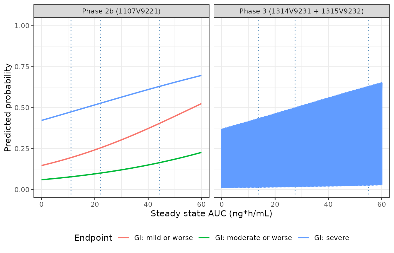
Replicates Kubota 2018 Supplemental Figure S6: probability of an SBM response and of a gastrointestinal disorder at each severity threshold, as a function of steady-state AUC. Vertical lines mark the mean AUCss at each dose (Supplemental Table S4 / Table VI convention).
# Structural properties of the fitted set, all deterministic.
shape <- curves |>
  dplyr::group_by(Model) |>
  dplyr::summarise(
    increasing = Probability[dplyr::n()] > Probability[1],
    in_unit = all(Probability >= 0 & Probability <= 1),
    .groups = "drop"
  )

stopifnot(all(shape$increasing), all(shape$in_unit))

# The three severity thresholds are CUMULATIVE, so within a study set the
# mild-or-worse curve must dominate moderate-or-worse, which must dominate
# severe. The authors fitted them independently, with no proportional-odds
# constraint, so this ordering is a property of the estimates rather than of
# the parameterisation -- worth checking rather than assuming.
ord <- curves |>
  dplyr::filter(grepl("^gi_", Model), grepl("Phase 3", Phase)) |>
  dplyr::select(Model, AUCss, Probability) |>
  tidyr::pivot_wider(names_from = Model, values_from = Probability)

stopifnot(
  all(ord$gi_mild_phase3 >= ord$gi_moderate_phase3),
  all(ord$gi_moderate_phase3 >= ord$gi_severe_phase3)
)
The paper’s headline safety claim
Kubota 2018 concludes that at 0.2 mg “the probability of the occurrence of severe gastrointestinal disorders was predicted to be less than 3%”, and that the same holds at 0.1 and 0.4 mg.
severe <- predict_er(er[["Kubota_2018_naldemedine_gi_severe_phase3"]], auc_p3)
names(severe) <- c("0 mg", "0.1 mg", "0.2 mg", "0.4 mg")
print(round(100 * severe, 2))
#>   0 mg 0.1 mg 0.2 mg 0.4 mg
#>   1.22   1.50   1.84   2.75

sbm_p3 <- predict_er(er[["Kubota_2018_naldemedine_sbm_phase3"]], auc_p3[3])
cat(sprintf("Predicted SBM responder probability at 0.2 mg (phase 3): %.1f%%\n", 100 * sbm_p3))
#> Predicted SBM responder probability at 0.2 mg (phase 3): 49.9%

stopifnot(
  # "less than 3%" at every studied dose -- deterministic, from the paper's
  # own predicted exposures.
  all(severe < 0.03),
  # "approximately 50%" SBM responders at 0.2 mg.
  abs(sbm_p3 - 0.50) < 0.02
)
End to end: the PK model feeds the exposure-response models
The two layers are connected in the source analysis by the individual AUCss. Here the simulated cohort’s NCA exposures are pushed through the phase 3 efficacy and severe-safety models, which is the operation Kubota 2018 performed with empirical Bayes estimates.
endtoend <- auc_check |>
  dplyr::select(id, arm, AUCss = auc) |>
  dplyr::mutate(
    p_sbm = predict_er(er[["Kubota_2018_naldemedine_sbm_phase3"]], AUCss),
    p_severe = predict_er(er[["Kubota_2018_naldemedine_gi_severe_phase3"]], AUCss)
  )

endtoend |>
  dplyr::group_by(Arm = arm) |>
  dplyr::summarise(
    `Median AUCss` = round(stats::median(AUCss), 2),
    `Mean P(SBM responder)` = round(mean(p_sbm), 3),
    `Mean P(severe GI)` = round(mean(p_severe), 4),
    .groups = "drop"
  ) |>
knitr::kable(caption = "Cohort-average predicted probabilities from PK-simulated steady-state exposures, phase 3 models.")| Arm | Median AUCss | Mean P(SBM responder) | Mean P(severe GI) |
|---|---|---|---|
| 0.1 mg | 11.78 | 0.428 | 0.0148 |
| 0.2 mg | 25.19 | 0.502 | 0.0190 |
| 0.4 mg | 47.66 | 0.617 | 0.0290 |
stopifnot(
  nrow(endtoend) == nrow(cohort),
  all(endtoend$p_sbm > 0 & endtoend$p_sbm < 1),
  # The efficacy relationship is shallow by construction; the claim under test
  # is that quadrupling the dose moves the responder probability by a modest
  # amount, not that it is flat. Cohort-derived, so gated on the mean with
  # headroom rather than on any subject.
  mean(endtoend$p_sbm[endtoend$arm == "0.4 mg"]) > mean(endtoend$p_sbm[endtoend$arm == "0.1 mg"]),
  mean(endtoend$p_severe) < 0.05
)
This is the quantitative basis for the paper’s conclusion. The covariate extremes move AUCss by -25% to +76% (checked above), and over that exposure range the responder probability changes by only a few percentage points while the severe-event probability stays under 3%. That is why Kubota 2018 concludes no covariate-driven dose adjustment is required.
Assumptions and deviations
The race indicator’s polarity is inverted relative to its name
This is the one reading in the paper that could plausibly have been taken the other way, and it is load-bearing: it decides which group carries a 13% clearance difference.
Kubota 2018’s Table III equation multiplies CL/F by
THETA(4)^White, which reads as “0.870 applies to White
subjects”. The Table II footnote says the opposite: “White = 1 for
non-White, White = 0 for White”. The indicator is named for the category
it excludes.
The footnote is correct, and the paper settles it in its own Results
text. The reference population – the subject at which every indicator is
zero, and whose CL/F is therefore THETA(1) unmodified – is described as
“52-year-old, 76 kg male, white, non-cancer, OIC patients with CLcr of
108 ml/min, administered under fasted condition”, with CL/F = 9.10 L/h.
That subject is White and carries no race factor, so
White = 0 for White subjects and the 0.870 applies to
non-White. The reference-subject anchor check above is the mechanical
gate on this: it solves a RACE_WHITE = 1 subject and
requires CL/F within 0.05% of 9.10. Under the equation-as-printed
reading the same subject would return 9.10 x 0.870 = 7.92 L/h, a 13%
miss that blows the gate by a factor of 260.
The covariate-extremes check is not what decides this, despite being the more tempting argument: the paper’s extremes let each covariate vary independently, so the free optimum simply attaches the 0.870 to whichever race label minimises CL/F, and both codings reproduce 5.17 and 12.1 L/h. It pins the continuous terms, not the polarity.
The model file therefore carries the published 0.870 unchanged and
raises it to the power (1 - RACE_WHITE), so the canonical
RACE_WHITE column keeps its usual polarity and the
inversion is visible at the call site.
Health status is carried on two ratified canonical columns
The source codes a three-level health status (healthy / chronic
non-cancer pain with OIC / cancer with OIC) with two indicator
variables, in which healthy subjects are the cell where both vanish.
Rather than mint a new canonical for “chronic non-cancer pain with OIC”,
the model carries the ratified DIS_HEALTHY and
DIS_CANCER columns and recovers the source’s
non-Cancer indicator inside model() as
(1 - DIS_HEALTHY) * (1 - DIS_CANCER). Encode a subject as
healthy with DIS_HEALTHY = 1, DIS_CANCER = 0; as
chronic-non-cancer-pain OIC with both 0; as cancer OIC with
DIS_CANCER = 1.
The body-weight exponent on Vc/F is fixed at 1, not estimated
Table III writes the age and creatinine-clearance terms as powers but
writes the weight term as * (Body weight/76) with no
exponent, so the exponent was held at 1 rather than estimated. The model
file encodes this as e_wt_vc <- fixed(1) so the
distinction between a fixed structural assumption and an estimate is not
lost.
Creatinine clearance is raw Cockcroft-Gault, not BSA-normalised
The CRCL canonical’s primary definition is
BSA-normalised mL/min/1.73 m^2, but Kubota 2018 uses a raw
Cockcroft-Gault clearance in mL/min (Methods, citing reference 12),
centred on the cohort median of 108 mL/min. Supplying a BSA-normalised
value to this model biases CL/F by (ratio)^0.0739. The
exponent is small, so the error is modest – but it is still an
error.
The creatinine-clearance effect’s confidence interval spans zero
The exponent 0.0739 has a 95% CI of -0.0133 to 0.161. Kubota 2018 retained the term despite this, because a dedicated renal-impairment study had shown a real AUC difference. That is a source-stated modelling decision and is reproduced unchanged rather than simplified away.
Inter-individual variability is diagonal
Kubota 2018 reports (Supplemental Figure S3) that “there was no clear
correlation between the inter-individual variabilities”, and publishes
no off-diagonal elements, so the omega matrix is diagonal.
Inter-individual variability on the absorption lag time was removed by
the authors to allow the estimation and covariance routines to converge,
so the model carries no etaltlag.
The IIV on Ka is very large
The published Ka CV of 161.2% is faithfully encoded, and it makes the simulated absorption phase extremely variable – a meaningful minority of subjects absorb slowly enough to be flip-flop. This is what the paper reports (with 32.6% shrinkage), not an artefact of the encoding, but it is why the NCA checks here gate AUC and its per-subject identity rather than Tmax or a terminal half-life, neither of which is stable across such a cohort.
The exposure-response models carry a placeholder residual error
The source fits are binomial logistic regressions in SAS with a
Bernoulli likelihood, which has no residual error parameter and no
random effects. Each exposure-response model file exposes a tiny fixed
additive residual (addSd_prob_* <- fixed(0.001)) purely
so the nlmixr2 observation machinery has an error model to attach to the
typical-value probability. That value is not from the
source and must not be interpreted as a published quantity.
Six of the seven exposure-response slopes have confidence intervals spanning zero
Only sbm_phase3 and gi_mild_phase3 have
slope confidence intervals excluding zero. Kubota 2018 is explicit about
this limitation: the exposure range studied spans only half to twice the
0.2 mg clinical dose, and the event counts at the stricter severity
thresholds are small. The paper’s own conclusion is that the models “can
be used to interpret the exposure response relationship” in these
studies but that “it is inappropriate to generalize them”. The models
are packaged as fitted; users extrapolating outside roughly 5 to 90
ng*h/mL should read that caveat first.
The exposure convention differs between Table VI and Table S4
Table VI’s 0.1 and 0.4 mg columns use AUCss values assumed
to be half and double the 0.2 mg value, not the observed means from
Supplemental Table S4 (11.06 versus 10.50, and 44.22 versus 43.76 in
phase 2b). Reproducing Table VI requires the assumed values;
characterising the fitted population requires the observed ones. Both
are recorded in the AUC_NALD register entry.
Equation 3’s raster is illegible in every available copy
The published PDF and the publisher’s supplementary figure files both
render Eq. (3) at a resolution too low to read. Its form was recovered
from two independent printed sources instead: the Table VI footnotes in
the PDF text layer, which spell it out as
Probability = 1 / [1 + exp(-a - b x AUCss)], and the
reproduction of all 28 Table VI cells above, which the same form
satisfies to the last printed decimal. No value was digitised from a
figure anywhere in this extraction.