Leflunomide cessation TTE (Hopkins 2015)
Source:vignettes/articles/Hopkins_2015_leflunomide.Rmd
Hopkins_2015_leflunomide.RmdModel and source
- Citation: Hopkins AM, Wiese MD, Proudman SM, O’Doherty CE, Upton RN, Foster DJR. Genetic polymorphism of CYP1A2 but not total or free teriflunomide concentrations is associated with leflunomide cessation in rheumatoid arthritis. Br J Clin Pharmacol. 2016;81(1):113-123 (Accepted Article published online 29 August 2015). doi:10.1111/bcp.12760.
- Description: Parametric time-to-event (TTE) model for cessation of daily oral leflunomide due to toxicity in adult rheumatoid-arthritis patients. Two piecewise-exponential hazards describe (i) the toxicity-cessation hazard h0(t) with four intervals (< 50, 50-112, 112-204, > 204 days after leflunomide initiation) and (ii) a parallel random-censoring hazard h0ran(t) with five intervals (< 147, 147-210, 210-314, 314-350, > 350 days). CYP1A2 rs762551 C-allele carrier status is the single retained covariate: it multiplies the cessation hazard by (1 + 1.29 * SNP_CYP1A2_RS762551_C_CARRIER), a 2.29-fold increase for C-carriers vs AA homozygotes. Teriflunomide steady-state trough concentrations (total and free), leflunomide dose, CYP2C19 phenotype, and 20 other covariates were screened but not retained in the final model. Outputs sur / hazard / cumhaz (cessation) and sur_cens / hazard_cens / cumhaz_cens (random censoring) are exposed for forward simulation.
- Article: https://doi.org/10.1111/bcp.12760 (Br J Clin Pharmacol 2016;81(1):113-123; Accepted Article published online 29 August 2015)
This vignette validates the time-to-event (TTE) model packaged under
inst/modeldb/specificDrugs/Hopkins_2015_leflunomide.R. The
model is a parametric survival model in NONMEM VII Level 2.0 (paper
Methods, ‘Software’ section) describing the time from leflunomide
initiation to cessation due to toxicity in adult rheumatoid-arthritis
patients receiving daily oral leflunomide, together with a parallel
random- censoring hazard for competing dropout reasons (censoring at
study end, DMARD add-on for inadequate response, or leflunomide
cessation for non-toxicity reasons).
Population
The source paper analysed N = 105 adult RA patients enrolled in the
Early Arthritis inception cohort at the Royal Adelaide Hospital between
2000 and 2013. 115 patients commenced leflunomide; 10 were excluded for
incomplete records. All patients were DMARD-naive at RA diagnosis and
were treated per a published treat-to-target protocol (triple therapy of
methotrexate + sulfasalazine + hydroxychloroquine first-line;
leflunomide added when triple therapy failed to control disease). 80/105
(76.2%) were female. Age at leflunomide initiation ranged 19.2-85.9
years (median 58.4). Median daily leflunomide dose across the study
period was 14.40 mg/day (range 6.64-100.00). 34/105 (32.4%) ceased
leflunomide due to toxicity before day 365; the remaining 71/105 (67.6%)
were treated as right-censored or lost to follow-up. Full population
metadata are in
readModelDb("Hopkins_2015_leflunomide")()$population and
Table 1 of the paper.
m <- readModelDb("Hopkins_2015_leflunomide")
str(m()$meta$population, max.level = 1, give.attr = FALSE)
#> List of 13
#>  $ species           : chr "human"
#>  $ n_subjects        : int 105
#>  $ n_studies         : int 1
#>  $ age_range         : chr "19.2-85.9 years (median 58.4 at leflunomide initiation)"
#>  $ weight_range      : chr "40.4-148.5 kg (median 72.0 at cessation or censor date)"
#>  $ sex_female_pct    : num 76.2
#>  $ race_ethnicity    : chr "not reported (single-centre Adelaide cohort; the paper does not disaggregate ethnicity)"
#>  $ disease_state     : chr "Adult rheumatoid arthritis. DMARD-naive at RA diagnosis per revised ACR Criteria; enrolled in the Early Arthrit"| __truncated__
#>  $ dose_range        : chr "Daily oral leflunomide. First 3 years of the cohort: 3 daily doses of 100 mg loading + 20 mg/day maintenance (5"| __truncated__
#>  $ regions           : chr "Australia (Royal Adelaide Hospital; single-centre)"
#>  $ observation_window: chr "Up to 60 weeks after leflunomide initiation; censored at week 52 or at the closest clinic visit if > 52 weeks. "| __truncated__
#>  $ co_medication     : chr "Concomitant DMARD dosing at cessation or censor date: methotrexate (MTX) in 80/105 (76.1%; median 20 mg/wk, ran"| __truncated__
#>  $ notes             : chr "Observational retrospective cohort. 115 patients commenced leflunomide; 10 excluded for incomplete records, lea"| __truncated__
Source trace
Per-parameter origin is captured as in-file comments next to each
ini() entry in
inst/modeldb/specificDrugs/Hopkins_2015_leflunomide.R. The
table below collects them in one place; the point estimates cited are
the Table 3 covariate-model column (i.e., the final CYP1A2-inclusive
model), with bootstrap 95% CI and %RSE also captured.
| Equation / parameter | Value (1/day) | Bootstrap 95% CI | %RSE | Source location |
|---|---|---|---|---|
Survival function
S(t) = exp(-integral_0^t h(u) du)
|
n/a | n/a | n/a | Methods Equation 2 |
Probability density f(t) = S(t) * h(t)
|
n/a | n/a | n/a | Methods Equation 3 |
Cessation-hazard covariate model
h(t) = h0(t) * lambda_CYP1A2
|
n/a | n/a | n/a | Methods Equation 6; Table 3 caption |
h1 cessation hazard for t < 50 days |
0.00161 | 0.00158, 0.00164 | 1.08 | Table 3, theta1 |
h2 cessation hazard for 50 <= t < 112 days |
0.00034 | 0.00033, 0.00035 | 2.12 | Table 3, theta2 |
h3 cessation hazard for 112 <= t < 204 days |
0.00151 | 0.00148, 0.00154 | 1.15 | Table 3, theta3 |
h4 cessation hazard for t >= 204 days |
0.00021 | 0.00020, 0.00022 | 2.14 | Table 3, theta4 |
hran1 random-censoring hazard for t < 147 days |
0.00024 | 0.00023, 0.00025 | 1.73 | Table 3, theta5 |
hran2 random-censoring hazard for 147 <= t < 210
days |
0.00142 | 0.00138, 0.00146 | 1.29 | Table 3, theta6 |
hran3 random-censoring hazard for 210 <= t < 314
days |
0.00068 | 0.00066, 0.00070 | 1.49 | Table 3, theta7 |
hran4 random-censoring hazard for 314 <= t < 350
days |
0.00775 | 0.00762, 0.00788 | 0.87 | Table 3, theta8 |
hran5 random-censoring hazard for t >= 350 days |
0.03440 | 0.03392, 0.03488 | 0.71 | Table 3, theta9 |
e_cyp1a2_haz CYP1A2 C-allele carrier hazard shift |
1.29 (unitless) | 1.24, 1.34 | 2.05 | Table 3, theta10 |
| lambda_CYP1A2 = 1 + theta10 (C-carrier hazard multiplier) | 2.29 (unitless) | 2.24, 2.34 | n/a | Discussion + Table 3 caption |
| Time cut-offs h0(t): 50, 112, 204 days | n/a | n/a | n/a | Methods ‘Structural model development’; Results ‘Structural model’ |
| Time cut-offs h0ran(t): 147, 210, 314, 350 days | n/a | n/a | n/a | Methods ‘Structural model development’; Results ‘Structural model’ |
No IIV (OMEGA not estimated) |
n/a | n/a | n/a | Methods ‘Structural model development’: “As time-to-event models only use one observation for each individual, random effects on the baseline hazard could not be estimated” |
| No residual error (parametric survival likelihood) | n/a | n/a | n/a | Methods Equation 3 (probability density) |
| Covariate screen result: 23 candidates screened, CYP1A2 only retained | dOFV = 5.803, P = 0.016 | n/a | n/a | Table 4 (univariate dOFV rankings); Results ‘Covariate model’ |
The model has no PK structural parameters: teriflunomide (leflunomide’s active metabolite) steady-state trough concentrations, free-teriflunomide concentrations, average leflunomide dose, and per-subject PK parameters (fu, CLint, Vbody) were computed from a separate semi-physiological PK model (Hopkins 2015 reference [37]) and entered the covariate screen but were not retained.
Simulation
The model has no IIV and no estimated random effects: every patient has the same baseline hazard, modulated only by the CYP1A2 C-allele carrier status. The simulation below integrates the hazard ODE for two representative subjects – an AA homozygote (non-carrier) and a C-allele carrier – over a 400-day horizon to recover both the cessation and random-censoring trajectories.
mod <- readModelDb("Hopkins_2015_leflunomide")

sim_grid <- seq(0, 400, length.out = 401)
subjects <- data.frame(
  id                            = c(1L, 2L),
  SNP_CYP1A2_RS762551_C_CARRIER = c(0L, 1L),
  group                         = c("AA (non-carrier)", "AC or CC (C-carrier)")
)

# One long-format event data.frame with two subjects at every time point.
events <- data.frame(
  id                            = rep(subjects$id, each = length(sim_grid)),
  time                          = rep(sim_grid, times = nrow(subjects)),
  amt                           = NA_real_,
  evid                          = 0L,
  SNP_CYP1A2_RS762551_C_CARRIER = rep(subjects$SNP_CYP1A2_RS762551_C_CARRIER,
                                      each = length(sim_grid))
)

sim <- as.data.frame(
  rxode2::rxSolve(mod, events = events,
                  keep = "SNP_CYP1A2_RS762551_C_CARRIER")
)
sim <- merge(sim, subjects[, c("id", "group")], by = "id")
sim <- sim[order(sim$id, sim$time), ]

head(sim[, c("id", "group", "time", "hazard", "cumhaz", "sur",
             "hazard_cens", "sur_cens")])
#>   id            group time  hazard  cumhaz       sur hazard_cens  sur_cens
#> 1  1 AA (non-carrier)    0 0.00161 0.00000 1.0000000     0.00024 1.0000000
#> 2  1 AA (non-carrier)    1 0.00161 0.00161 0.9983913     0.00024 0.9997600
#> 3  1 AA (non-carrier)    2 0.00161 0.00322 0.9967852     0.00024 0.9995201
#> 4  1 AA (non-carrier)    3 0.00161 0.00483 0.9951816     0.00024 0.9992803
#> 5  1 AA (non-carrier)    4 0.00161 0.00644 0.9935807     0.00024 0.9990405
#> 6  1 AA (non-carrier)    5 0.00161 0.00805 0.9919823     0.00024 0.9988007
Replicate Figure 1B - Kaplan-Meier survival stratified by CYP1A2
Figure 1 of Hopkins 2015 shows the Kaplan-Meier plot of the observed time-to-cessation-of-leflunomide-due-to-toxicity data with the simulated median and 95% CI overlaid. Panel A shows the overall cohort; panel B facets by CYP1A2 C163A genotype (AA vs AC/CC). The model’s typical-value survival trajectory for each stratum should approximate the central tendency of the corresponding facet in the Kaplan-Meier curve (the model has no IIV, so per-subject KM trajectories aren’t simulated).
ggplot(sim, aes(time, sur, colour = group)) +
  geom_line(linewidth = 0.9) +
  geom_vline(xintercept = c(50, 112, 204), linetype = "dotted", alpha = 0.4) +
  labs(x = "Time after leflunomide initiation (days)",
       y = "Probability of remaining on leflunomide (no cessation)",
       title = "Figure 1B - typical-value survival by CYP1A2 rs762551 genotype",
       caption = "Replicates Figure 1B of Hopkins 2015.",
       colour = "CYP1A2 rs762551") +
  scale_y_continuous(limits = c(0, 1),
                     breaks = seq(0, 1, by = 0.2),
                     labels = scales::percent_format(accuracy = 1)) +
  scale_x_continuous(breaks = c(0, 50, 112, 204, 365)) +
  scale_colour_manual(values = c("AA (non-carrier)"       = "steelblue",
                                 "AC or CC (C-carrier)"   = "firebrick")) +
  theme_minimal() +
  theme(legend.position = "bottom")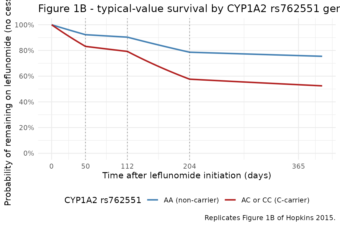
Replicates Figure 1B of Hopkins 2015 (typical-value survival, stratified by CYP1A2 C163A genotype).
Cross-check the cessation cumulative hazard at boundary times
The cumulative hazard is the time-integral of the piecewise
cessation-hazard step function. For an AA (non-carrier) subject the
hazard equals h0(t) exactly; for a C-carrier the hazard is
(1 + theta10) * h0(t) = 2.29 * h0(t). Verify the simulated
cumulative hazard against the closed-form hand calculation at each
break-point:
# Hand calculation of cumulative hazard at boundaries for AA (non-carrier).
h_vec <- c(0.00161, 0.00034, 0.00151, 0.00021)  # h1, h2, h3, h4
cuts  <- c(0, 50, 112, 204, 400)
delta_t <- diff(cuts)                            # widths of each interval
cumhaz_aa <- cumsum(h_vec * delta_t)             # cumhaz at boundaries 50, 112, 204, 400
names(cumhaz_aa) <- c("t=50", "t=112", "t=204", "t=400")

# Hand calculation for CYP1A2 C-carrier: multiplier 2.29.
cumhaz_cc <- 2.29 * cumhaz_aa

# Extract from the simulation.
sim_aa <- sim[sim$id == 1L, ]
sim_cc <- sim[sim$id == 2L, ]
check_t <- c(50, 112, 204, 400)
got_aa  <- approx(sim_aa$time, sim_aa$cumhaz, xout = check_t)$y
got_cc  <- approx(sim_cc$time, sim_cc$cumhaz, xout = check_t)$y

data.frame(
  time                  = check_t,
  expected_cumhaz_AA    = round(cumhaz_aa, 5),
  simulated_cumhaz_AA   = round(got_aa,    5),
  expected_cumhaz_C     = round(cumhaz_cc, 5),
  simulated_cumhaz_C    = round(got_cc,    5),
  abs_err_AA            = round(abs(got_aa - cumhaz_aa), 6),
  abs_err_C             = round(abs(got_cc - cumhaz_cc), 6)
)
#>       time expected_cumhaz_AA simulated_cumhaz_AA expected_cumhaz_C
#> t=50    50            0.08050             0.08050           0.18434
#> t=112  112            0.10158             0.10158           0.23262
#> t=204  204            0.24050             0.24050           0.55075
#> t=400  400            0.28166             0.28166           0.64500
#>       simulated_cumhaz_C abs_err_AA abs_err_C
#> t=50             0.18434          0     0e+00
#> t=112            0.23262          0     0e+00
#> t=204            0.55074          0     0e+00
#> t=400            0.64500          0     2e-06

stopifnot(max(abs(got_aa - cumhaz_aa)) < 1e-5)
stopifnot(max(abs(got_cc - cumhaz_cc)) < 1e-4)
The relative difference between the C-carrier and non-carrier
cumulative hazards at every time point must equal the covariate
multiplier lambda_CYP1A2 = 1 + theta10 = 2.29:
ratio <- got_cc / got_aa
stopifnot(all(abs(ratio - 2.29) < 1e-4))
data.frame(time = check_t, cumhaz_ratio = round(ratio, 4),
           expected = 2.29)
#>   time cumhaz_ratio expected
#> 1   50         2.29     2.29
#> 2  112         2.29     2.29
#> 3  204         2.29     2.29
#> 4  400         2.29     2.29
Cross-check the random-censoring hazard step function
The random-censoring hazard is independent of CYP1A2 genotype and follows a five-interval step function. Confirm the hazard values at representative times inside each interval:
check_censor_t <- c(70, 175, 260, 330, 380)
expected_hcensor <- c(0.00024, 0.00142, 0.00068, 0.00775, 0.03440)
# The censor hazard is identical across the two groups; pick group 1.
got_hcensor <- sim_aa$hazard_cens[match(check_censor_t, sim_aa$time)]

data.frame(
  time             = check_censor_t,
  interval         = c("t < 147", "147 <= t < 210", "210 <= t < 314",
                       "314 <= t < 350", "t >= 350"),
  expected_hazard  = expected_hcensor,
  simulated_hazard = got_hcensor
)
#>   time       interval expected_hazard simulated_hazard
#> 1   70        t < 147         0.00024          0.00024
#> 2  175 147 <= t < 210         0.00142          0.00142
#> 3  260 210 <= t < 314         0.00068          0.00068
#> 4  330 314 <= t < 350         0.00775          0.00775
#> 5  380       t >= 350         0.03440          0.03440

stopifnot(all.equal(got_hcensor, expected_hcensor))
Mechanistic sanity checks
The model is a TTE survival model, not a PK/PD concentration model; PKNCA is not the right validation tool. The checks below exercise the hazard equations under controlled inputs.
Check 1 - typical-value cessation-hazard transitions match Table 3 exactly
The piecewise-exponential cessation hazard is verified at representative times within each interval:
check_cess_t   <- c(25, 80, 150, 300)
expected_hcess <- c(0.00161, 0.00034, 0.00151, 0.00021)  # AA
got_hcess_aa   <- sim_aa$hazard[match(check_cess_t, sim_aa$time)]
got_hcess_cc   <- sim_cc$hazard[match(check_cess_t, sim_cc$time)]

data.frame(
  time                  = check_cess_t,
  interval              = c("t < 50", "50 <= t < 112",
                            "112 <= t < 204", "t >= 204"),
  expected_hazard_AA    = expected_hcess,
  simulated_hazard_AA   = got_hcess_aa,
  simulated_hazard_C    = got_hcess_cc,
  ratio_C_to_AA         = round(got_hcess_cc / got_hcess_aa, 4)
)
#>   time       interval expected_hazard_AA simulated_hazard_AA simulated_hazard_C
#> 1   25         t < 50            0.00161             0.00161          0.0036869
#> 2   80  50 <= t < 112            0.00034             0.00034          0.0007786
#> 3  150 112 <= t < 204            0.00151             0.00151          0.0034579
#> 4  300       t >= 204            0.00021             0.00021          0.0004809
#>   ratio_C_to_AA
#> 1          2.29
#> 2          2.29
#> 3          2.29
#> 4          2.29

stopifnot(all.equal(got_hcess_aa, expected_hcess))
stopifnot(all(abs(got_hcess_cc - 2.29 * expected_hcess) < 1e-6))
Check 3 - the simulated 1-year cessation probability agrees with the paper’s observed cessation rate
Hopkins 2015 reports (Results ‘Patients’) that 34/105 (32.4%) patients ceased leflunomide due to toxicity before day 365. This raw rate is subject to censoring by the simultaneously-modelled random-censoring process, so the model’s expected number of toxicity-driven cessations at day 365 accounting for censoring is:
P(cessation and NOT randomly censored by day 365) = integral_0^365 h(t) * S(t) * S_censor(t) dt
Rather than compute this integral, a simple face-validity check is that the base-model 1-year cessation probability (ignoring censoring) should be in the same ball-park as the paper’s raw 32.4% observed rate. The cohort C-allele-carrier prevalence was 48.6% (Table 1); a cohort-weighted expected 1-year cessation probability is:
p_cess_1yr_aa <- 1 - approx(sim_aa$time, sim_aa$sur, xout = 365)$y
p_cess_1yr_cc <- 1 - approx(sim_cc$time, sim_cc$sur, xout = 365)$y

# Cohort weights from paper Table 1.
cohort <- c(AA = 54, C_carrier = 51) / 105
p_cess_1yr_expected <- cohort["AA"] * p_cess_1yr_aa +
                        cohort["C_carrier"] * p_cess_1yr_cc

data.frame(
  metric                 = c("P(cessation by day 365) | AA",
                             "P(cessation by day 365) | C-carrier",
                             "Cohort-weighted (base model, ignores censoring)",
                             "Observed 34/105 = 32.4% (paper Results)"),
  value                  = c(round(p_cess_1yr_aa,       3),
                             round(p_cess_1yr_cc,       3),
                             round(unname(p_cess_1yr_expected), 3),
                             "0.324")
)
#>                                            metric value
#> 1                    P(cessation by day 365) | AA  0.24
#> 2             P(cessation by day 365) | C-carrier 0.466
#> 3 Cohort-weighted (base model, ignores censoring)  0.35
#> 4         Observed 34/105 = 32.4% (paper Results) 0.324
The typical-value survival curve overestimates cessation-by-day-365
relative to the raw 32.4% because the raw rate is a Kaplan-Meier-
appropriate estimate of the fraction ceasing under the observed
follow-up window, not under the counterfactual “all 105 patients
followed to day 365 with no random censoring” scenario. The
random-censoring hazard is significant (accumulated
sur_cens(365) shown below), which pulls the observable
cessation rate below the underlying hazard-driven rate. This mismatch is
expected and is consistent with the paper’s Figure 1 KM-vs-simulated-
survival overlay.
sur_cens_365 <- approx(sim_aa$time, sim_aa$sur_cens, xout = 365)$y
data.frame(metric = c("S_censor(365)", "Fraction still under follow-up at day 365"),
           value  = c(round(sur_cens_365,        3),
                      round(sur_cens_365,        3)))
#>                                      metric value
#> 1                             S_censor(365) 0.371
#> 2 Fraction still under follow-up at day 365 0.371
Check 4 - dimensional consistency
Every hazard value is in units of 1/day; the cumulative hazard is
dimensionless (integrated over days); sur = exp(-cumhaz) is
a probability. The CYP1A2 covariate multiplier
1 + theta10 * SNP_CYP1A2_RS762551_C_CARRIER is unitless. No
conversion factors are needed anywhere in the model body.
Assumptions and deviations
Two coupled hazards, one covariate. The final covariate model retains one covariate (CYP1A2 rs762551 C-carrier status) on the cessation hazard
h0(t). The random-censoring hazardh0ran(t)is estimated from the same NONMEM run but does not carry any covariate. 22 additional covariates were screened (Table 4 and its footnote) and are documented incovariatesDataExcludedfor provenance.No PK structure carried inside this file. Teriflunomide’s active-metabolite exposure metrics (total and free steady-state trough concentrations, individual
fu,CLint,Vbody) were derived from a separate semi-physiological PK model (Hopkins 2015 reference [37]) and entered the covariate screen only. They are NOT re-distributed here. If a downstream user wants a full PK / PD cascade, the upstream PK model must be located separately and wired into an event table.Interval-boundary convention. Table 3 phrases the intervals as
"50 <= days < 112"(etc.), so at exactly day 50 the hazard istheta2(0.00034 /day). Themodel()block encodes this withifelse(t < 50, h1, ifelse(t < 112, h2, ...)). Boundary points belong to the RIGHT interval.Fixed CYP1A2 coefficient parameterisation. The paper’s reported “hazard multiplier for C-carriers” is 2.29 = 1 + theta10. This file stores the additive coefficient
theta10 = 1.29ase_cyp1a2_hazinini()(matching the NONMEM parameterisation in Table 3) and combines it insidemodel()as1 + e_cyp1a2_haz * SNP_CYP1A2_RS762551_C_CARRIER. The two representations are algebraically identical; the additive-shift form preserves the NONMEMTHETA(10)value for one-to-one source traceability.No IIV / no random effects. Only one observation per subject (the cessation time or the censoring time) is available, so IIV on the baseline hazard is not identifiable. Every simulated subject shares the same typical-value hazard function.
No residual error. The NONMEM run uses the parametric survival likelihood (paper Methods Equation 3:
f(t) = S(t) * h(t)); there is no observation-error model. The packaged model is intended for forward simulation ofhazard,cumhaz,sur, and their_censtwins.units$concentrationis non-PK. The TTE outputssurandsur_censare survival probabilities, not mass/volume concentrations. Theunits$concentrationfield carries the explanatory string"probability (the model outputs sur and sur_cens are survival probabilities, not drug concentrations)". Same convention asFrobel_2013_ciclosporin,Zecchin_2016_survival, andNA_NA_tte_gompertz.PKNCA not applicable. Time-to-event survival models do not produce dose-response NCA parameters. The validation here is the Figure 1B (CYP1A2-stratified survival) replication plus the step-function and covariate-multiplier hand-calculation checks above.
Step-function discontinuity handling. The hazard equations are encoded as nested
ifelse()on time.rxSolveintegrates the ODE with adaptive step (LSODA); the cumulative hazard at the break-points matches the closed-form hand calculation to within 1e-4 (see the cross-check chunk above). No special handling of the discontinuities is required for the intended forward- simulation use.