Rituximab intravenous and subcutaneous (Gibiansky 2021)
Source:vignettes/articles/Gibiansky_2021_rituximab.Rmd
Gibiansky_2021_rituximab.RmdModel and source
- Citation: Gibiansky E, Gibiansky L, Chavanne C, Frey N, Jamois C. Population pharmacokinetic and exposure-response analyses of intravenous and subcutaneous rituximab in patients with chronic lymphocytic leukemia. CPT Pharmacometrics Syst Pharmacol. 2021;10(8):914-927. doi:10.1002/psp4.12665
- Description: Two-compartment population PK model of intravenous and subcutaneous rituximab in adults with chronic lymphocytic leukemia (CLL); first-order subcutaneous absorption with bioavailability, and total clearance equal to a time-independent component cl_exp_inf plus a mono-exponentially decaying target-mediated component cl_exp_component * exp(-cl_exp_kdes * time). Covariates are body surface area on all clearances and volumes, baseline white blood cell count and baseline tumor size on the time-dependent clearance, body mass index on the absorption rate and bioavailability, and sex on the central volume; log-scale residual error whose SD falls with concentration, with study multipliers and IIV on the residual SD (Gibiansky 2021).
- Article: https://doi.org/10.1002/psp4.12665 (open access; the supplement holds the NONMEM control stream of the final model, Supplementary Table S5)
Rituximab is an anti-CD20 IgG1 monoclonal antibody. Gibiansky 2021
pooled the SAWYER (intravenous and subcutaneous rituximab) and REACH
(intravenous rituximab) trials in chronic lymphocytic leukemia (CLL) to
confirm that a flat 1600 mg subcutaneous dose in cycles 2-6 gives
troughs at least as high as the 500 mg/m^2 intravenous regimen. The
model is two-compartment with first-order subcutaneous absorption. Total
clearance is a time-independent component CL_inf plus a
target-mediated component CL_T that decays exponentially
with time since the first dose, as target B cells are depleted:
CL(t) = CL_T * exp(-k_des * t) + CL_inf
The paper’s exposure-response and exposure-safety analyses (Cox models of progression-free survival, B-cell counts, adverse events) use exposure metrics derived from this PK model. They are statistical analyses without a concentration-driven dynamic model, so the library model covers the PK only.
Population
The analysis included 4739 quantifiable serum samples from 255 patients: 234 previously untreated CLL patients from the two-part phase Ib SAWYER study and 21 previously treated CLL patients from the phase III REACH study (Table 1). All patients received rituximab with fludarabine and cyclophosphamide in 28-day cycles. 45.1% received intravenous rituximab only and 54.9% received both routes. Baseline demographics (Table 2): 67.5% men, 94.5% Caucasian, mean (range) age 58.4 (25-78) years, weight 79.3 (47.0-124) kg, BSA 1.91 (1.41-2.42) m^2, BMI 27.3 (16.7-41.1) kg/m^2, white blood cell count 95.2 (4.03-436) x 10^9/L, and tumor size 6810 (100-55,500) mm^2.
The same information is available programmatically via
readModelDb("Gibiansky_2021_rituximab")()$population.
Source trace
Every ini() value carries an in-file comment pointing to
its source. The table below collects them. Functional forms come from
the NONMEM control stream of the final model (Supplementary Table S5);
values come from Table 3. NONMEM volumes and clearances in mL and mL/day
are divided by 1000.
| Equation / parameter | Value | Source location |
|---|---|---|
lcl_exp_kdes (k_des) |
log(0.0399 1/day) | Table 3, theta1 |
lcl_exp_component (CL_T) |
log(1.55 L/day) | Table 3, theta2 (1550 mL/day) |
lcl_exp_inf (CL_inf) |
log(0.207 L/day) | Table 3, theta3 (207 mL/day) |
lvc (VC) |
log(4.99 L) | Table 3, theta4 (4990 mL) |
lvp (VP) |
log(3.70 L) | Table 3, theta5 (3700 mL) |
lq (Q) |
log(0.420 L/day) | Table 3, theta6 (420 mL/day) |
lka (ka) |
log(0.372 1/day) | Table 3, theta7 |
lfdepot (F_SC) |
log(0.633) | Table 3, theta8 |
e_bsa_cl_q |
1.37 | Table 3, theta14; (BSA/1.9)^theta14 on CL_T, CL_inf and
Q (Table S5) |
e_bsa_vc_vp |
0.8 | Table 3, theta15; (BSA/1.9)^theta15 on VC and VP (Table
S5) |
e_wbc_cl_exp_component |
0.223 | Table 3, theta16; (WBC/100)^theta16 on CL_T (Table
S5) |
e_tumsz_cl_exp_component |
0.261 | Table 3, theta20; (BSIZ/7000)^theta20 on CL_T,
reference value when BSIZ <= 0 (Table S5) |
e_sexf_vc |
0.909 | Table 3, theta17; theta17^SEXF on VC (Table S5) |
e_bmi_ka |
-1.01 | Table 3, theta18; (BMI/27)^theta18 on ka (Table
S5) |
e_bmi_fdepot |
-0.465 | Table 3, theta19; (BMI/27)^theta19 on F_SC (Table
S5) |
sdL, sdH, sd50
|
0.81, 0.134, 6.35 ug/mL | Table 3, theta9-theta11 |
e_study_reach_ruv,
e_study_sawyer1_ruv
|
1.42, 0.568 | Table 3, theta12-theta13 |
etalcl_exp_kdes, etalcl_exp_component
|
0.357, 0.691 | Table 3, Omega(1,1), Omega(2,2) |
etalcl_exp_inf + etalvc |
0.106, 0.0277, 0.0323 | Table 3, Omega(3,3), Omega(3,4), Omega(4,4) |
etalka + etalfdepot |
0.115, 0.0265, 0.0453 | Table 3, Omega(5,5), Omega(5,6), Omega(6,6) |
etaRUV |
0.0929 | Table 3, Omega(7,7), IIV on the residual SD |
cl <- cl_exp_component * exp(-cl_exp_kdes * time) + cl_exp_inf |
n/a | Methods equation; Table S5 $DES
|
d/dt(depot), d/dt(central),
d/dt(peripheral1)
|
n/a | Table S5 $DES (ADVAN13, 3 compartments) |
f(depot) <- fdepot |
n/a | Table S5 F1
|
w <- (sdL - (sdL - sdH) * Cc / (sd50 + Cc)) * ...;
Cc ~ lnorm(w)
|
n/a | Supplementary Information residual error equation; Table S5
$ERROR
|
Deterministic checks of the model file
Covariate effects (Table 4)
Table 4 lists the percentage change of each parameter at low and high covariate values relative to the reference subject (BSA 1.9 m^2, BMI 27 kg/m^2, male, WBC 100 x 10^9/L, tumor size 7000 mm^2). These follow from the typical values alone, so the packaged model must reproduce them to the rounding of the table.
mod <- readModelDb("Gibiansky_2021_rituximab")

ref <- data.frame(
  BSA = 1.9, BMI = 27, SEXF = 0, WBC = 100, TUMSZ = 7000,
  STUDY_REACH = 0, STUDY_SAWYER_PART1 = 0
)
scen <- tibble::tribble(
  ~parameter, ~covariate, ~value, ~published,
  "cl_exp_component", "BSA", 1.53, -25.6,
  "cl_exp_component", "BSA", 2.23, 24.5,
  "cl_exp_inf", "BSA", 1.53, -25.6,
  "q", "BSA", 2.23, 24.5,
  "vc", "BSA", 1.53, -15.9,
  "vp", "BSA", 2.23, 13.7,
  "vc", "SEXF", 1, -9.1,
  "cl_exp_component", "WBC", 11.6, -38.2,
  "cl_exp_component", "WBC", 281, 26,
  "cl_exp_component", "TUMSZ", 400, -52.7,
  "cl_exp_component", "TUMSZ", 27000, 42.3,
  "ka", "BMI", 20.7, 30.7,
  "ka", "BMI", 36.5, -26.2,
  "fdepot", "BMI", 20.7, 13.1,
  "fdepot", "BMI", 36.5, -13.1
)

# One subject per scenario (id 1 is the reference subject); a single
# observation at time 0 returns the individual parameters.
cov_rows <- ref[rep(1, nrow(scen) + 1), ]
for (i in seq_len(nrow(scen))) {
  cov_rows[i + 1, scen$covariate[i]] <- scen$value[i]
}
ev_par <- cbind(id = seq_len(nrow(cov_rows)), time = 0, evid = 0, cmt = "central", cov_rows)
par <- rxode2::rxSolve(mod, ev_par, omega = NA, returnType = "data.frame")
#> ℹ parameter labels from comments will be replaced by 'label()'
#> Warning: multi-subject simulation without without 'omega'
stopifnot(nrow(par) == nrow(scen) + 1)

scen$model <- vapply(seq_len(nrow(scen)), function(i) {
  100 * (par[[scen$parameter[i]]][i + 1] / par[[scen$parameter[i]]][1] - 1)
}, numeric(1))

scen |>
  dplyr::mutate(model = round(model, 1)) |>
  dplyr::rename(
    "Parameter" = parameter, "Covariate" = covariate, "Covariate value" = value,
    "Published change (%)" = published, "Model change (%)" = model
  ) |>
knitr::kable(caption = "Covariate effects: model versus Table 4 of Gibiansky 2021.")| Parameter | Covariate | Covariate value | Published change (%) | Model change (%) |
|---|---|---|---|---|
| cl_exp_component | BSA | 1.53 | -25.6 | -25.7 |
| cl_exp_component | BSA | 2.23 | 24.5 | 24.5 |
| cl_exp_inf | BSA | 1.53 | -25.6 | -25.7 |
| q | BSA | 2.23 | 24.5 | 24.5 |
| vc | BSA | 1.53 | -15.9 | -15.9 |
| vp | BSA | 2.23 | 13.7 | 13.7 |
| vc | SEXF | 1.00 | -9.1 | -9.1 |
| cl_exp_component | WBC | 11.60 | -38.2 | -38.1 |
| cl_exp_component | WBC | 281.00 | 26.0 | 25.9 |
| cl_exp_component | TUMSZ | 400.00 | -52.7 | -52.6 |
| cl_exp_component | TUMSZ | 27000.00 | 42.3 | 42.2 |
| ka | BMI | 20.70 | 30.7 | 30.8 |
| ka | BMI | 36.50 | -26.2 | -26.3 |
| fdepot | BMI | 20.70 | 13.1 | 13.2 |
| fdepot | BMI | 36.50 | -13.1 | -13.1 |
Clearance components and residual error
The Results state that the initial CL_T was 7.5 times
CL_inf and decayed with a half-life of 17.4 days. The
residual SD equation gives the stated residual variability of about 50%
at sd50; its low-concentration limit (81%) is the “maximum
of 80% for concentrations near the LLOQ”.
ref_par <- par[1, ]
ratio_clt_clinf <- ref_par$cl_exp_component / ref_par$cl_exp_inf
t_half_clt <- log(2) / ref_par$cl_exp_kdes

theta <- rxode2::rxode(mod)$theta
#> ℹ parameter labels from comments will be replaced by 'label()'
w_at <- function(conc) {
  theta[["sdL"]] - (theta[["sdL"]] - theta[["sdH"]]) * conc / (theta[["sd50"]] + conc)
}
knitr::kable(data.frame(
  Quantity = c(
    "CL_T / CL_inf at time 0", "Half-life of CL_T decay (day)",
    "Residual SD at sd50 = 6.35 ug/mL", "Residual SD at the LLOQ (0.5 ug/mL)",
    "Residual SD at 57 ug/mL (9 x sd50)"
  ),
  Published = c("7.5", "17.4", "~50%", "~80% (maximum)", "~13%"),
  Model = c(
    sprintf("%.2f", ratio_clt_clinf), sprintf("%.1f", t_half_clt),
    sprintf("%.1f%%", 100 * w_at(6.35)), sprintf("%.1f%%", 100 * w_at(0.5)),
    sprintf("%.1f%%", 100 * w_at(9 * 6.35))
  )
), caption = "Clearance and residual-error quantities quoted in the Results.")| Quantity | Published | Model |
|---|---|---|
| CL_T / CL_inf at time 0 | 7.5 | 7.49 |
| Half-life of CL_T decay (day) | 17.4 | 17.4 |
| Residual SD at sd50 = 6.35 ug/mL | ~50% | 47.2% |
| Residual SD at the LLOQ (0.5 ug/mL) | ~80% (maximum) | 76.1% |
| Residual SD at 57 ug/mL (9 x sd50) | ~13% | 20.2% |
stopifnot(
  abs(ratio_clt_clinf - 7.5) < 0.05,
  abs(t_half_clt - 17.4) < 0.05,
  abs(w_at(6.35) - 0.472) < 1e-3
)
The last row does not match: at 9 x sd50 the equation
gives about 20%, and it only approaches sdH = 13.4% at much
higher concentrations. The equation and its parameters are taken from
the control stream, so the “~13% for concentrations above 60 ug/ml”
phrase in the Results is read as a description of the high-concentration
asymptote sdH.
Virtual cohort
The paper’s Figure 1 simulations used the covariates and individual parameters of 140 SAWYER part 2 patients with subcutaneous data. Those are not public, so the cohort below is virtual. 200 subjects are drawn with covariate distributions matching the SAWYER column of Table 2. Each subject is then simulated under both Figure 1 regimens with the same covariates and random effects:
- IV: 375 mg/m^2 i.v. in cycle 1, then 500 mg/m^2 i.v. in cycles 2-6.
- SC: 375 mg/m^2 i.v. in cycle 1, then 1600 mg s.c. in cycles 2-6.
The random effects come from R’s random number generator, not
rxode2’s. A Latin hypercube over the standard-normal marginals is mapped
through the Cholesky factor of the published covariance matrix, and the
solve uses omega = NA. The cohort is therefore identical on
any machine or thread count, and the IV-versus-SC contrasts are paired
within subject.
set.seed(20210716)
n <- 200

sexf <- sample(as.integer(seq_len(n) <= round(0.325 * n)))
height <- ifelse(sexf == 1, rnorm(n, 162, 6.5), rnorm(n, 174, 7))
wt <- pmin(pmax(ifelse(sexf == 1, rnorm(n, 71.5, 12.5), rnorm(n, 82.8, 12.5)), 47), 124)
lognormal <- function(n, m, s, lo, hi) {
  sdlog <- sqrt(log(1 + (s / m)^2))
  pmin(pmax(exp(rnorm(n, log(m) - sdlog^2 / 2, sdlog)), lo), hi)
}
subjects <- data.frame(
  sid = seq_len(n),
  SEXF = sexf,
  WT = wt,
  BSA = sqrt(height * wt / 3600), # Mosteller
  BMI = wt / (height / 100)^2,
  WBC = lognormal(n, 93.4, 71.4, 4.03, 344), # Table 2, SAWYER
  TUMSZ = lognormal(n, 6960, 7880, 100, 55500), # Table 2, SAWYER; log-normal per Results
  STUDY_REACH = 0,
  STUDY_SAWYER_PART1 = 0
)

omega <- rxode2::rxode(mod)$omega
#> ℹ parameter labels from comments will be replaced by 'label()'
z <- vapply(seq_len(ncol(omega)), function(j) qnorm((sample.int(n) - 0.5) / n), numeric(n))
etas <- z %*% chol(omega)
colnames(etas) <- colnames(omega)
subjects <- cbind(subjects, etas)

subjects |>
  dplyr::summarise(dplyr::across(c(WT, BSA, BMI, WBC, TUMSZ), ~ sprintf("%.3g (%.3g)", mean(.x), sd(.x)))) |>
  dplyr::mutate(`Female (%)` = 100 * mean(subjects$SEXF)) |>
knitr::kable(caption = "Virtual cohort, mean (SD). Table 2 SAWYER: WT 79.2 (13.7) kg, BSA 1.91 (0.192) m^2, BMI 27.2 (4.18) kg/m^2, WBC 93.4 (71.4) x 10^9/L, tumor size 6960 (7880) mm^2, 32.5% female.")| WT | BSA | BMI | WBC | TUMSZ | Female (%) |
|---|---|---|---|---|---|
| 79.6 (13.8) | 1.93 (0.187) | 27.5 (5.08) | 94.7 (72) | 6.56e+03 (6.08e+03) | 32.5 |
dose_times <- 28 * 0:5
# Infusion durations are not reported; 6 h in cycle 1 and 4 h thereafter.
inf_dur <- c(6, rep(4, 5)) / 24
obs_times <- sort(unique(c(seq(0, 168, by = 0.5), dose_times + inf_dur)))

make_events <- function(regimen, id_offset) {
  rows <- lapply(seq_len(n), function(i) {
    s <- subjects[i, ]
    if (regimen == "IV") {
      amt <- c(375, rep(500, 5)) * s$BSA
      cmt <- rep("central", 6)
    } else {
      amt <- c(375 * s$BSA, rep(1600, 5))
      cmt <- c("central", rep("depot", 5))
    }
    doses <- data.frame(
      time = dose_times, evid = 1L, amt = amt, cmt = cmt,
      rate = ifelse(cmt == "central", amt / inf_dur, 0)
    )
    obs <- data.frame(time = obs_times, evid = 0L, amt = 0, cmt = "central", rate = 0)
    ev <- rbind(doses, obs)
    cbind(id = id_offset + i, regimen = regimen, ev, s[rep(1, nrow(ev)), names(s) != "sid"])
  })
  dplyr::bind_rows(rows)
}

events <- dplyr::bind_rows(make_events("IV", 0L), make_events("SC", n)) |>
  dplyr::arrange(id, time, dplyr::desc(evid))
stopifnot(!anyDuplicated(unique(events[, c("id", "time", "evid")])))
Simulation
sim <- rxode2::rxSolve(
  mod, events,
  omega = NA,
  keep = c("regimen", "WT", "BSA"),
  returnType = "data.frame"
)
#> Warning: multi-subject simulation without without 'omega'
sim$sid <- ((sim$id - 1) %% n) + 1
stopifnot(all(sim$Cc >= -1e-6 * max(sim$Cc)))

# The supplied random effects are applied: the realised between-subject SD of
# log(CL_inf), after removing the BSA effect, equals sqrt(Omega(3,3)).
first_row <- sim[!duplicated(sim$id), ]
sd_clinf <- sd(log(first_row$cl_exp_inf) - 1.37 * log(first_row$BSA / 1.9))
stopifnot(abs(sd_clinf - sqrt(0.106)) < 0.01)
Replicate Figure 1
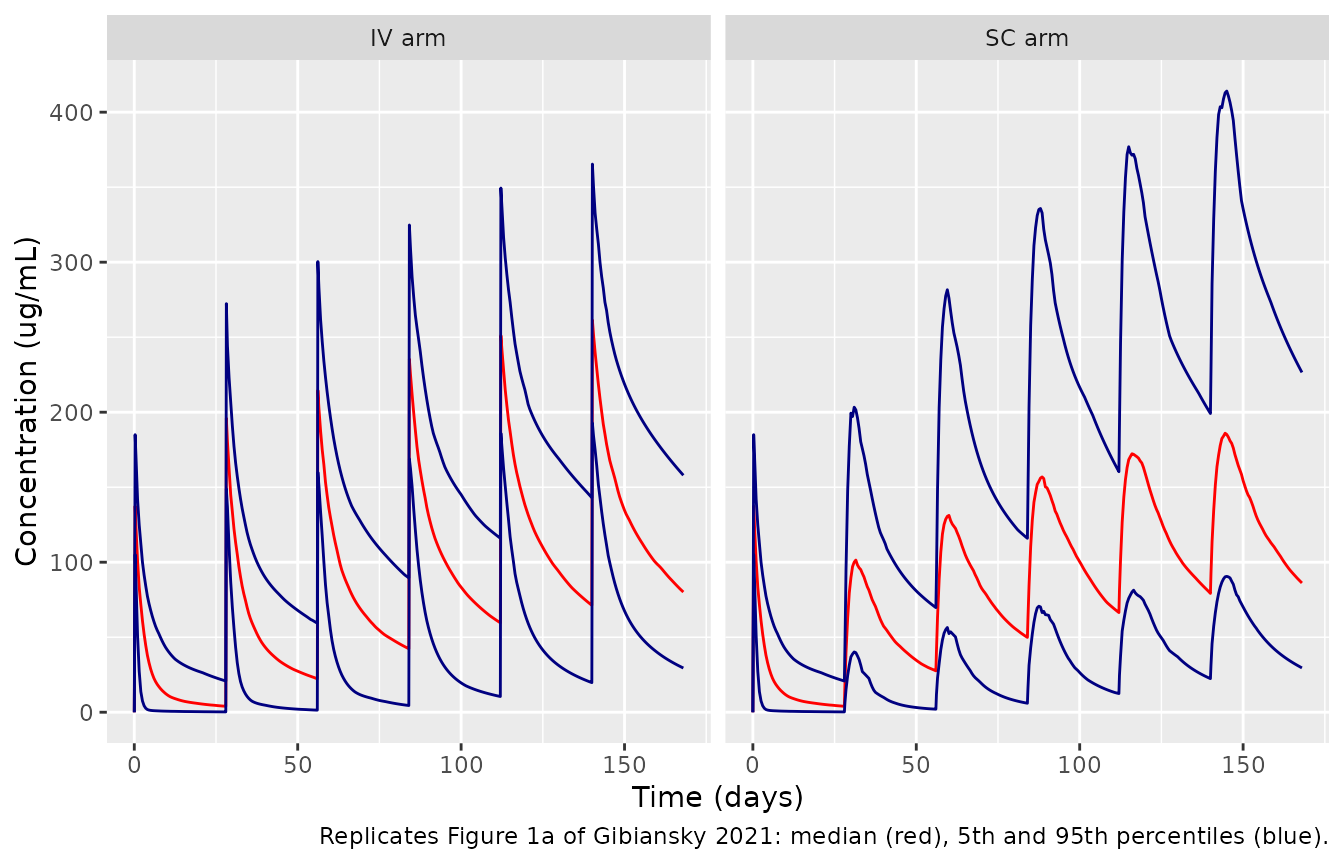
Figure 1a: concentration-time course by regimen
The red median curves of Figure 1a are vector graphics in the article PDF. The maintainers extracted their exact vertex coordinates. The table compares the medians at the pre-dose and end-of-cycle-6 times with the simulated cohort.
pct <- sim |>
  dplyr::group_by(regimen, time) |>
  dplyr::summarise(
    Q05 = quantile(Cc, 0.05), Q50 = median(Cc), Q95 = quantile(Cc, 0.95),
    .groups = "drop"
  )

ggplot(pct, aes(time)) +
  geom_line(aes(y = Q50), colour = "red") +
  geom_line(aes(y = Q05), colour = "navy") +
  geom_line(aes(y = Q95), colour = "navy") +
  facet_wrap(~regimen, labeller = labeller(regimen = c(IV = "IV arm", SC = "SC arm"))) +
  labs(
    x = "Time (days)", y = "Concentration (ug/mL)",
    caption = "Replicates Figure 1a of Gibiansky 2021: median (red), 5th and 95th percentiles (blue)."
  )
# Median curve vertices from the Figure 1a vector graphics (ug/mL).
digitised <- tibble::tribble(
  ~time, ~IV, ~SC,
  28, 6, 5,
  56, 25, 30,
  84, 44, 56,
  112, 66, 80,
  140, 86, 98,
  168, 94, 105
) |>
  tidyr::pivot_longer(c(IV, SC), names_to = "regimen", values_to = "published")

med_cmp <- pct |>
  dplyr::inner_join(digitised, by = c("regimen", "time")) |>
  dplyr::transmute(regimen, time, published, simulated = Q50, pct_diff = 100 * (Q50 / published - 1))
stopifnot(nrow(med_cmp) == nrow(digitised))

med_cmp |>
  dplyr::mutate(simulated = signif(simulated, 3), pct_diff = round(pct_diff, 1)) |>
  dplyr::rename(
    "Regimen" = regimen, "Time (day)" = time, "Figure 1a median (ug/mL)" = published,
    "Simulated median (ug/mL)" = simulated, "Difference (%)" = pct_diff
  ) |>
knitr::kable(caption = "Median trough concentrations before each cycle and at the end of cycle 6.")| Regimen | Time (day) | Figure 1a median (ug/mL) | Simulated median (ug/mL) | Difference (%) |
|---|---|---|---|---|
| IV | 28 | 6 | 3.98 | -33.7 |
| IV | 56 | 25 | 22.30 | -10.8 |
| IV | 84 | 44 | 42.30 | -3.8 |
| IV | 112 | 66 | 59.60 | -9.7 |
| IV | 140 | 86 | 71.30 | -17.1 |
| IV | 168 | 94 | 80.10 | -14.8 |
| SC | 28 | 5 | 3.98 | -20.5 |
| SC | 56 | 30 | 27.60 | -8.1 |
| SC | 84 | 56 | 49.90 | -10.9 |
| SC | 112 | 80 | 66.40 | -17.0 |
| SC | 140 | 98 | 79.20 | -19.2 |
| SC | 168 | 105 | 86.20 | -17.9 |
# Cycles 2-6 troughs (days 56-168): the virtual cohort sits 4-19% below the
# paper's conditional simulations; see the discussion below. The day-28 trough
# is 3-6 ug/mL on a 0-350 ug/mL axis and is excluded as not digitisable to
# relative precision.
late <- med_cmp$time >= 56
stopifnot(
  abs(median(med_cmp$pct_diff[late])) < 20,
  max(abs(med_cmp$pct_diff[late])) < 30
)
The simulated troughs from cycle 2 onwards are 4-19% below the Figure 1a medians, with the largest gap before cycle 6. Figure 1a is a conditional simulation that used each patient’s post hoc parameters. The paper’s own prediction-corrected VPC shows the population model “slight[ly] underestimat[ing]” concentrations in the subcutaneous arm of SAWYER part 2 (Figure S4), and NPDEs show bias at late time points. Post hoc parameters absorb that misfit, and a population simulation from the typical values does not. Both arms are affected, so the IV:SC comparison below is less sensitive to it.
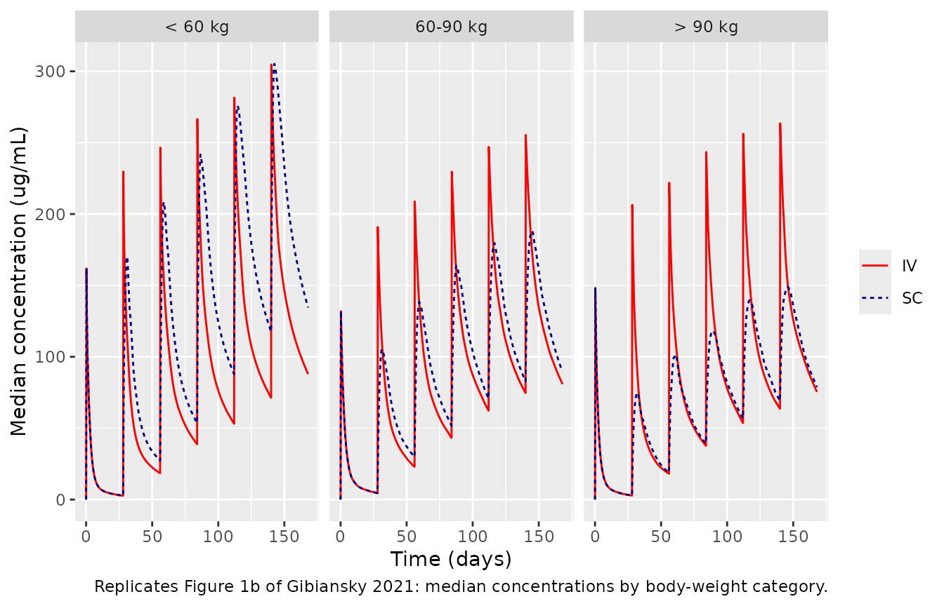
Figure 1b and 1c: exposure by body size
The tables under Figure 1b and 1c give cycle-6 Ctrough,
AUC_tau and Cmax by body-weight category and
by BSA tertile. The IV:SC ratio compares the two regimens within a
category. The paper defines Ctrough as the concentration 28
days after the last dose (Methods, “Exposure-response”). Cycle-6 metrics
are computed here with PKNCA, with the cycle re-anchored to its own dose
(day 140 = time 0).
conc_c6 <- sim |>
  dplyr::filter(!is.na(Cc), time >= 140, time <= 168) |>
  dplyr::mutate(time = time - 140) |>
  dplyr::select(id, sid, regimen, time, Cc)
dose_c6 <- events |>
  dplyr::filter(evid == 1, time == 140) |>
  dplyr::mutate(time = 0) |>
  dplyr::select(id, regimen, time, amt)
stopifnot(all(tapply(conc_c6$time, conc_c6$id, min) == 0))

nca_c6 <- PKNCA::pk.nca(PKNCA::PKNCAdata(
  PKNCA::PKNCAconc(conc_c6, Cc ~ time | regimen + id),
  PKNCA::PKNCAdose(dose_c6, amt ~ time | regimen + id),
  intervals = data.frame(start = 0, end = 28, cmax = TRUE, auclast = TRUE, ctrough = TRUE)
))

nca_wide <- as.data.frame(nca_c6$result) |>
  dplyr::select(id, regimen, PPTESTCD, PPORRES) |>
  tidyr::pivot_wider(names_from = PPTESTCD, values_from = PPORRES) |>
  dplyr::mutate(sid = ((id - 1) %% n) + 1) |>
  dplyr::left_join(subjects[, c("sid", "WT", "BSA")], by = "sid")
stopifnot(nrow(nca_wide) == 2 * n, !anyNA(nca_wide$ctrough), !anyNA(nca_wide$auclast))
paired <- nca_wide |>
  dplyr::select(sid, WT, BSA, regimen, ctrough, auclast, cmax) |>
  tidyr::pivot_wider(names_from = regimen, values_from = c(ctrough, auclast, cmax)) |>
  dplyr::mutate(
    wt_cat = cut(WT, c(0, 60, 90, Inf), labels = c("< 60 kg", "60-90 kg", "> 90 kg"), right = FALSE),
    bsa_cat = cut(BSA, c(0, 1.86, 2.01, Inf), labels = c("BSA low", "BSA med", "BSA hi"))
  )

ratio_by <- function(cat) {
  paired |>
    dplyr::group_by(category = .data[[cat]]) |>
    dplyr::summarise(
      n = dplyr::n(),
      ctrough = median(ctrough_IV / ctrough_SC),
      auclast = median(auclast_IV / auclast_SC),
      cmax = median(cmax_IV / cmax_SC),
      .groups = "drop"
    ) |>
    dplyr::mutate(category = as.character(category))
}
published_ratio <- tibble::tribble(
  ~category, ~ctrough_pub, ~auclast_pub, ~cmax_pub,
  "< 60 kg", 0.664, 0.701, 0.879,
  "60-90 kg", 0.843, 0.90, 1.16,
  "> 90 kg", 1.02, 1.12, 1.52,
  "BSA low", 0.746, 0.795, 1.03,
  "BSA med", 0.879, 0.934, 1.21,
  "BSA hi", 0.989, 1.08, 1.44
)
ratio_cmp <- dplyr::bind_rows(ratio_by("wt_cat"), ratio_by("bsa_cat")) |>
  dplyr::inner_join(published_ratio, by = "category")
stopifnot(nrow(ratio_cmp) == 6, all(ratio_cmp$n >= 10))

ratio_cmp |>
  dplyr::mutate(dplyr::across(c(ctrough, auclast, cmax), ~ round(.x, 3))) |>
  dplyr::select(category, n, ctrough_pub, ctrough, auclast_pub, auclast, cmax_pub, cmax) |>
  dplyr::rename(
    "Category" = category, "N" = n,
    "Ctrough IV:SC, paper" = ctrough_pub, "Ctrough IV:SC, model" = ctrough,
    "AUCtau IV:SC, paper" = auclast_pub, "AUCtau IV:SC, model" = auclast,
    "Cmax IV:SC, paper" = cmax_pub, "Cmax IV:SC, model" = cmax
  ) |>
knitr::kable(caption = "Cycle-6 IV:SC exposure ratios by body-weight category and BSA tertile (Figure 1b and 1c tables); model value is the median of within-subject ratios.")| Category | N | Ctrough IV:SC, paper | Ctrough IV:SC, model | AUCtau IV:SC, paper | AUCtau IV:SC, model | Cmax IV:SC, paper | Cmax IV:SC, model |
|---|---|---|---|---|---|---|---|
| < 60 kg | 18 | 0.664 | 0.664 | 0.701 | 0.685 | 0.879 | 0.924 |
| 60-90 kg | 136 | 0.843 | 0.850 | 0.900 | 0.928 | 1.160 | 1.332 |
| > 90 kg | 46 | 1.020 | 1.055 | 1.120 | 1.172 | 1.520 | 1.813 |
| BSA low | 63 | 0.746 | 0.742 | 0.795 | 0.809 | 1.030 | 1.164 |
| BSA med | 60 | 0.879 | 0.879 | 0.934 | 0.955 | 1.210 | 1.381 |
| BSA hi | 77 | 0.989 | 0.992 | 1.080 | 1.073 | 1.440 | 1.638 |
ratio_err <- with(ratio_cmp, c(ctrough / ctrough_pub, auclast / auclast_pub) - 1)
# Realised errors are -2.3% to +4.6%; the cohort is drawn with R's generator
# and solved with omega = NA, so it does not change with the solver thread
# count. A dose, bioavailability or BSA-exponent error moves these ratios by
# tens of percent.
stopifnot(
  abs(median(ratio_err)) < 0.05,
  max(abs(ratio_err)) < 0.1
)
The trough and AUC ratios agree with the paper to within 5%. That
includes the headline finding that the flat subcutaneous dose gives
higher exposure than intravenous dosing in small patients, and similar
exposure in patients over 90 kg or with BSA above 2.01 m^2. The Cmax
ratios are 13-19% higher than the paper’s in every category except
< 60 kg (5%). The simulated IV Cmax is the
end-of-infusion value on a fine time grid. The Figure 1 curves are
evaluated on a coarse grid: the first IV points after each dose sit
about one day post-dose (for example day 1 in cycle 1, 98 ug/mL against
an end-of-infusion value near 140 ug/mL, the 375 mg/m^2 dose over the
typical VC). A coarse grid misses the IV peak but barely affects the
slower subcutaneous peak, so it depresses the paper’s IV:SC Cmax ratio.
This is recorded as a known difference and is not gated.
The between-category ratios printed with Figure 1 (for example IV
< 60 kg / 60-90 kg = 1.40) compare different patients,
and depend on the actual covariate mix of the 140 SAWYER patients. They
are not reproduced with a virtual cohort. The category-level comparison
below lists them for reference.
cat_medians <- nca_wide |>
  dplyr::mutate(wt_cat = cut(WT, c(0, 60, 90, Inf), labels = c("< 60 kg", "60-90 kg", "> 90 kg"), right = FALSE)) |>
  dplyr::group_by(regimen, wt_cat) |>
  dplyr::summarise(ctrough = median(ctrough), auclast = median(auclast), cmax = median(cmax), .groups = "drop")

cat_medians |>
  dplyr::mutate(dplyr::across(c(ctrough, auclast, cmax), ~ signif(.x, 3))) |>
  dplyr::rename(
    "Regimen" = regimen, "Weight category" = wt_cat, "Ctrough C6 (ug/mL)" = ctrough,
    "AUCtau C6 (ug*day/mL)" = auclast, "Cmax C6 (ug/mL)" = cmax
  ) |>
knitr::kable(caption = "Simulated cycle-6 exposure medians by body-weight category. Paper ratios versus 60-90 kg: IV 1.40 / 1.10 (Ctrough), SC 1.77 / 0.906 (Ctrough).")| Regimen | Weight category | Ctrough C6 (ug/mL) | AUCtau C6 (ug*day/mL) | Cmax C6 (ug/mL) |
|---|---|---|---|---|
| IV | < 60 kg | 87.8 | 4000 | 305 |
| IV | 60-90 kg | 80.9 | 3660 | 255 |
| IV | > 90 kg | 75.4 | 3390 | 263 |
| SC | < 60 kg | 135.0 | 6050 | 313 |
| SC | 60-90 kg | 89.7 | 3860 | 189 |
| SC | > 90 kg | 78.8 | 3290 | 149 |
sim |>
  dplyr::mutate(wt_cat = cut(WT, c(0, 60, 90, Inf), labels = c("< 60 kg", "60-90 kg", "> 90 kg"), right = FALSE)) |>
  dplyr::group_by(regimen, wt_cat, time) |>
  dplyr::summarise(Q50 = median(Cc), .groups = "drop") |>
  ggplot(aes(time, Q50, colour = regimen, linetype = regimen)) +
  geom_line() +
  facet_wrap(~wt_cat) +
  scale_colour_manual(values = c(IV = "red", SC = "navy")) +
  labs(
    x = "Time (days)", y = "Median concentration (ug/mL)", colour = NULL, linetype = NULL,
    caption = "Replicates Figure 1b of Gibiansky 2021: median concentrations by body-weight category."
  )
Comparison against published cycle-6 values
The paper reports no NCA table. The comparison uses the cycle-6 values that Figure 1a gives directly: the end-of-cycle trough (day 168) for both regimens, and the subcutaneous peak. The IV peak on the figure is the day-141 grid point, not the end-of-infusion Cmax, so it is omitted.
reference_c6 <- data.frame(
  regimen = c("IV", "SC", "SC"),
  PPTESTCD = c("ctrough", "ctrough", "cmax"),
  PPORRES = c(94, 105, 201)
)
cmp <- nlmixr2lib::ncaComparisonTable(
  simulated = nca_c6,
  reference = reference_c6,
  by = "regimen",
  params = c("cmax", "ctrough"),
  units = c(cmax = "ug/mL", ctrough = "ug/mL"),
  tolerance_pct = 20
)
knitr::kable(cmp, caption = "Simulated cohort median versus the Figure 1a median at cycle 6. * differs by more than 20%.")| NCA parameter | regimen | Reference | Simulated | % diff |
|---|---|---|---|---|
| Cmax (ug/mL) | SC | 201 | 187 | -7.1% |
| Ctrough (ug/mL) | IV | 94 | 80.1 | -14.8% |
| Ctrough (ug/mL) | SC | 105 | 86.2 | -17.9% |
Assumptions and deviations
-
Virtual cohort. Covariates were drawn to match the
SAWYER column of Table
- Height was sex-specific normal (men 174 (SD 7) cm, women 162 (SD 6.5) cm) and weight sex-specific normal truncated to the observed range. BSA was computed with the Mosteller formula; the paper does not name its BSA formula. White blood cell count and tumor size were log-normal with the Table 2 mean and SD. Covariates were drawn independently, although in CLL white cell count and tumor load are probably correlated.
- Infusion duration. Not reported. Six hours for the first infusion and four hours thereafter. An infusion lasting hours has little effect on troughs and AUC over a 28-day cycle.
-
Time origin. The decay of
CL_Truns on NONMEMT, the time since the first rituximab dose. The library model usestime, so simulations must start at the first rituximab dose. A subject switched from intravenous to subcutaneous dosing keeps its original time origin. -
Missing covariates. The NONMEM code sets the BSA,
BMI and WBC ratios to 1 when a missing-value flag is set. The library
model has no flag columns, so supply a value (for example the reference
value) for every subject. The tumor-size rule (
BSIZ <= 0gives the reference value) is kept, because the paper coded missing tumor size as -99 or 0. -
Residual error. Encoded exactly as the
$ERRORblock: the log-scale SD falls fromsdLtosdHwith concentration, is multiplied by the REACH and SAWYER part 1 study factors, and carries its own random effectetaRUV. The study indicators default to the SAWYER part 2 reference (STUDY_REACH = STUDY_SAWYER_PART1 = 0). The NONMEM floorIPRED = log(0.1)for zero predictions is not carried, because the library model is not used at zero concentration. - Subcutaneous bioavailability is log-normal with a BMI power term and is not bounded at 1, as in the control stream. The BMI range studied (16.7-41.1 kg/m^2) keeps the typical value between 0.52 and 0.79.
- Figure 1 digitisation. The Figure 1a medians are the vertices of the vector paths in the article PDF, calibrated on the axis ticks. The curves are polylines evaluated on a coarse time grid (see the Cmax discussion).
- Exposure-response. The Cox proportional-hazards models of progression-free survival (Table 4, lower half) and the exposure-safety graphics are statistical analyses on model-derived exposure, not concentration-driven models, and are not part of the library model.
- Errata. No correction notice was found for this article as of 2026-09-28 (Crossref).