Apixaban (Kolowrat 2025)
Source:vignettes/articles/Kolowrat_2025_apixaban.Rmd
Kolowrat_2025_apixaban.RmdModel and source
#> ℹ parameter labels from comments will be replaced by 'label()'Citation: Kolowrat S, Riley C, Lam K, Thomson L, Stickle DF, Kraft WK. Real-world impact of amiodarone on apixaban population pharmacokinetics in hospitalized patients. Clin Transl Sci. 2025;18(11):e70392. doi:10.1111/cts.70392. The fixed absorption rate constant ka = 0.82 1/h is inherited from Gaspar F, Terrier J, Favre S, et al. Population pharmacokinetics of apixaban in a real-life hospitalized population from the OptimAT study. CPT Pharmacometrics Syst Pharmacol. 2023;12(10):1541-1552. doi:10.1002/psp4.13032; see modellib(‘Gaspar_2023_apixaban’).
Description: One-compartment population pharmacokinetic model with first-order absorption and linear elimination for oral apixaban 2.5 or 5 mg twice daily in hospitalized adults with nonvalvular atrial fibrillation (Kolowrat 2025), quantifying the real-world amiodarone drug-drug interaction from salvaged clinical plasma samples. Apparent oral clearance CL/F = 1.5 L/h at the cohort median age of 77 years without amiodarone, scaled by a power function of age (AGE/77)^-1.52 and multiplied by exp(-0.4) = 0.670 (a 33% reduction, 95% CI 12% to 48%) during concomitant amiodarone 200 mg. Apparent volume of distribution V/F = 45.57 L carries no covariate. The absorption rate constant ka was fixed to 0.82 1/h from the Gaspar 2023 OptimAT apixaban model because its interindividual variability was imprecisely estimated and fixing it improved the corrected Bayesian information criterion; see modellib(‘Gaspar_2023_apixaban’). Interindividual variability is supported on CL/F (62.23% CV) and V/F (52.66% CV) but not on ka. Residual variability is combined proportional (15%) and additive (21.28 ng/mL). Two-compartment models were explored but the peripheral volume and intercompartmental clearance were not estimable from the sparse real-world data. Renal function (estimated glomerular filtration rate, creatinine clearance), body weight and body mass index were screened and not retained.
Article: https://doi.org/10.1111/cts.70392
Open access via Europe PMC: https://europepmc.org/article/MED/PMC12597975
Kolowrat 2025 asks a question that a conventional drug-drug interaction study cannot answer. Amiodarone’s half-life is about 50 days, so a crossover design in healthy volunteers is neither ethical nor feasible; instead the authors built a population PK model from salvaged plasma – samples drawn for routine clinical care that had passed a five-day discard threshold – in 106 hospitalized patients with nonvalvular atrial fibrillation, 51 of whom were on a stable dose of amiodarone 200 mg.
The model is deliberately simple: one compartment, first-order
absorption, no lag time, and only two retained covariates.
Two-compartment models were explored but the peripheral volume and
intercompartmental clearance were not estimable from the sparse
real-world data, and the interindividual variability on ka
was so imprecise that removing it improved the corrected Bayesian
information criterion by 7.37 units, with a further 9.48-unit
improvement from fixing ka outright to the value published
by Gaspar 2023.
Population
| Field | Value |
|---|---|
| Species | human |
| Subjects | 106 (55 apixaban alone, 51 apixaban + amiodarone) |
| Observations | 360 plasma samples, 7 below the 5 ng/mL limit of quantification |
| Median age | 77 years (overall cohort median, the centering value for the CL/F age term) |
| Age (by group) | IQR 71-86 years apixaban alone (median 79); IQR 64-83 years apixaban plus amiodarone (median 74). Full range not reported. |
| Median weight | 86.4 kg apixaban alone; 83.4 kg apixaban plus amiodarone |
| Female | 48.1% |
| Renal function | Median eGFR 48 mL/min/1.73 m^2 (CKD-EPI 2021) and median Cockcroft-Gault creatinine clearance about 38 mL/min in both groups; a renally impaired cohort |
| Co-medication | Concomitant amiodarone 200 mg in 51/106 (48.1%); mild / moderate CYP3A4 or P-gp perpetrators other than amiodarone in 31/106 (29.2%) |
| Region | United States (single-centre retrospective observational study, Thomas Jefferson University Hospital, Philadelphia, Pennsylvania; IRB iRISID-2023-2228, approved 6 December 2024) |
Two features of this cohort drive everything below. It is old – the group medians are 79 and 74 years and the interquartile ranges reach 86 – and it is renally impaired, with a median estimated glomerular filtration rate of 48 mL/min/1.73 m^2 and a median Cockcroft-Gault creatinine clearance near 38 mL/min in both arms. That is why the estimated apparent clearance of 1.5 L/h is well below the roughly 3.3 L/h typical of younger apixaban cohorts, and why the authors’ own comparison against Morath 2025 (Figure S5) shows this model predicting higher exposures.
The same information is available programmatically via
readModelDb("Kolowrat_2025_apixaban")()$population.
Source trace
The per-parameter origin is recorded as an in-file comment next to
each ini() entry in
inst/modeldb/specificDrugs/Kolowrat_2025_apixaban.R. The
table below collects them in one place for review.
| Parameter | Value | Source |
|---|---|---|
lka |
log(0.82), fixed | Table 2 final: Ka = 0.82 1/h (Fixed). Results 3.2 gives the provenance (Gaspar 2023, reference 22) and the reason (IIV on Ka imprecise; dBICc -9.48 on fixing). |
lcl |
log(1.5) | Table 2 final: CL/F = 1.5 L/h (RSE 8.99%, 95% CI 1.26-1.78). Intercept of the Table 2 note equation at AGE = 77, no amiodarone. |
lvc |
log(45.57) | Table 2 final: V/F = 45.57 L (RSE 10.6%, 95% CI 37.11-55.96). |
e_age_cl |
-1.52 | Table 2 final: beta_CL,age = -1.52 (RSE 25%, 95% CI -2.27 to -0.78). |
e_amio_cl |
-0.4 | Table 2 final: beta_CL,amio = -0.4 (RSE 33.8%, 95% CI -0.66 to -0.13). |
etalvc |
0.244754 | Table 2 final: IIV V = 52.66% CV (RSE 17.4%, omega CI 0.35-0.69); omega^2 = log(0.5266^2 + 1). |
etalcl |
0.327329 | Table 2 final: IIV CL = 62.23% CV (RSE 9.65%, omega CI 0.47-0.69); omega^2 = log(0.6223^2 + 1). |
propSd |
0.15 | Table 2 final: proportional error 0.15 (RSE 18.3%, 95% CI 0.11-0.21). |
addSd |
21.28 | Table 2 final: additive error 21.28 ng/mL (RSE 25.4%, 95% CI 13.21-34.26). |
| CL/F equation | n/a | Table 2 note: CL/F_i = 1.5 x (Age/77)^beta_age x e^(beta_amio x 1_{CAT=1}) x e^(IIV_CL/F_i). |
| Continuous covariate form | n/a | Methods 2.3: log(theta_i) = log(theta_pop) + beta_theta x log(COV_i / COV_median) + eta_theta,i. |
| Categorical covariate form | n/a | Methods 2.3: log(theta_i) = log(theta_pop) + beta_theta x 1_{CAT_i=1} + eta_theta,i. |
| One compartment, first-order absorption, no lag | n/a | Methods 2.2 and Results 3.2 (two-compartment models rejected: peripheral V and Q not supported). |
| Combined proportional + additive error | n/a | Methods 2.2 and Results 3.2 (selected over additive-only and proportional-only). |
How the interindividual-variability scale was pinned
Table 2 reports the interindividual variability as a percent CV
(52.66, 62.23) but reports the confidence
interval for the same row on the omega (standard deviation) scale
(0.35-0.69, 0.47-0.69) – two different scales
in one row. That makes the internal variance ambiguous on its face, so
it is worth showing how the ambiguity resolves rather than asserting
it.
Monolix computes confidence intervals for variance parameters on the
log scale, omega * exp(+/- 1.96 * RSE). Applying the
log-normal inversion omega = sqrt(log(CV^2 + 1)) reproduces
all eight printed bounds across the base and final
models; reading the CV column as omega directly misses six of them.
| Table 2 row | CV% | omega = sqrt(log(CV^2+1)) | variance used in ini() | CI from that omega | CI printed in Table 2 | CI if CV column were omega |
|---|---|---|---|---|---|---|
| V/F base | 52.58 | 0.49 | 0.24 | 0.361 - 0.676 | 0.36 - 0.67 | 0.384 - 0.719 |
| CL/F base | 69.91 | 0.63 | 0.40 | 0.528 - 0.754 | 0.53 - 0.75 | 0.585 - 0.835 |
| V/F final | 52.66 | 0.49 | 0.24 | 0.352 - 0.696 | 0.35 - 0.69 | 0.374 - 0.741 |
| CL/F final | 62.23 | 0.57 | 0.33 | 0.474 - 0.691 | 0.47 - 0.69 | 0.515 - 0.752 |
Model structure at a glance
| Age (years) | Amiodarone | CL/F (L/h) | V/F (L) | kel (1/h) | t1/2 (h) |
|---|---|---|---|---|---|
| 65 | no | 1.941 | 45.57 | 0.043 | 16.277 |
| 65 | yes | 1.301 | 45.57 | 0.029 | 24.283 |
| 77 | no | 1.500 | 45.57 | 0.033 | 21.058 |
| 77 | yes | 1.005 | 45.57 | 0.022 | 31.415 |
| 85 | no | 1.291 | 45.57 | 0.028 | 24.472 |
| 85 | yes | 0.865 | 45.57 | 0.019 | 36.507 |
The implied terminal half-life is 21 h for a typical 77-year-old without amiodarone and 31 h with it. That is notably longer than the roughly 12 h apixaban half-life the paper itself invokes in Methods 2.1 when it defines a 60 h (five half-life) washout window, and it follows directly from the low apparent clearance in this elderly, renally impaired cohort. It is a property of the published estimates, not a transcription artefact – see Assumptions and deviations.
Deterministic checks
These use rxode2::zeroRe() and steady-state dosing
(ss = 1), so they contain no random numbers at all and are
reproducible on any machine and any thread count. The tolerances are
therefore tight: they measure numerical error, not cohort sampling.
tau <- 12  # dosing interval (h), twice daily

# One steady-state dosing interval for a single typical subject. `ss = 1` with
# `ii = tau` asks rxode2 for the exact steady state, which avoids any question
# about whether a hand-built dosing train ran long enough (the longest half-life
# this model can produce, for an old subject on amiodarone with a low-CL eta, is
# over 100 h).
ss_events <- function(id, dose, age, amio, by = 0.05) {
  dplyr::bind_rows(
    data.frame(time = 0, amt = dose, evid = 1L, cmt = "depot",
               ss = 1L, ii = tau),
    data.frame(time = seq(0, tau, by = by), amt = NA_real_, evid = 0L,
               cmt = "central", ss = NA_integer_, ii = NA_real_)
  ) |>
    dplyr::mutate(id = id, AGE = age, CONMED_AMIO = amio) |>
    dplyr::arrange(time, dplyr::desc(evid))
}

mod_typical <- rxode2::zeroRe(ui)
Mass balance: AUC over one interval equals dose divided by clearance
For any linear model at steady state,
AUC[0,tau] = Dose / CL exactly. This is a genuine gate on
the ODE solution: the left-hand side comes from integrating the
central state that the solver produced, the right-hand side
from the individual clearance the covariate model computed. A wrong
kel, a mis-wired depot, or an absorption term that loses
mass all break it.
arms <- tibble::tribble(
  ~grp,              ~dose, ~amio, ~age_t1,
  "2.5 mg BID",        2.5,    0L,      79,
  "2.5 mg BID+amio",   2.5,    1L,      74,
  "5 mg BID",          5.0,    0L,      79,
  "5 mg BID+amio",     5.0,    1L,      74
)

ev_t1 <- dplyr::bind_rows(lapply(seq_len(nrow(arms)), function(i) {
  ss_events(i, arms$dose[i], arms$age_t1[i], arms$amio[i]) |>
    dplyr::mutate(grp = arms$grp[i], dose = arms$dose[i])
}))
# steady-state searches for long-half-life subjects exceed the default step budget
sim_t1 <- rxode2::rxSolve(mod_typical, events = ev_t1, keep = "grp",
                          maxsteps = 1e6) |>
  as.data.frame()
#> ℹ omega/sigma items treated as zero: 'etalvc', 'etalcl'
#> Warning: multi-subject simulation without without 'omega'

stopifnot(!any(is.na(sim_t1$Cc)), !any(is.nan(sim_t1$Cc)), all(sim_t1$Cc >= 0))

mb <- sim_t1 |>
  dplyr::filter(!is.na(Cc)) |>
  dplyr::group_by(grp) |>
  dplyr::summarise(
    cl_model = unique(cl),
    auc_ode  = PKNCA::pk.calc.auc(Cc, time, interval = c(0, tau), auc.type = "AUClast"),
    .groups  = "drop"
  ) |>
  dplyr::left_join(arms |> dplyr::select(grp, dose), by = "grp") |>
  dplyr::mutate(
    auc_closed = 1000 * dose / cl_model,
    pct        = 100 * (auc_ode - auc_closed) / auc_closed
  )

mb |>
  dplyr::select(grp, cl_model, auc_ode, auc_closed, pct) |>
  dplyr::rename(
    "Regimen"                 = grp,
    "CL/F (L/h)"              = cl_model,
    "AUCtau from ODE"         = auc_ode,
    "Dose / CL (closed form)" = auc_closed,
    "% difference"            = pct
  ) |>
  knitr::kable(digits = c(0, 4, 1, 1, 5),
caption = "Steady-state mass-balance identity, ng*h/mL.")| Regimen | CL/F (L/h) | AUCtau from ODE | Dose / CL (closed form) | % difference |
|---|---|---|---|---|
| 2.5 mg BID | 1.4427 | 1732.9 | 1732.9 | -0.00069 |
| 2.5 mg BID+amio | 1.0681 | 2340.6 | 2340.6 | -0.00061 |
| 5 mg BID | 1.4427 | 3465.8 | 3465.8 | -0.00069 |
| 5 mg BID+amio | 1.0681 | 4681.2 | 4681.3 | -0.00061 |
Dose linearity
The model carries no saturable term, so doubling the dose must exactly double every exposure metric at a fixed age.
ratio_noamio <- mb$auc_ode[mb$grp == "5 mg BID"]      / mb$auc_ode[mb$grp == "2.5 mg BID"]
ratio_amio   <- mb$auc_ode[mb$grp == "5 mg BID+amio"] / mb$auc_ode[mb$grp == "2.5 mg BID+amio"]
c(`no amiodarone` = ratio_noamio, `with amiodarone` = ratio_amio)
#>   no amiodarone with amiodarone
#>               2               2

stopifnot(abs(ratio_noamio - 2) < 1e-4, abs(ratio_amio - 2) < 1e-4)
The amiodarone effect reproduces the paper’s headline number
The abstract, Study Highlights, Results and Discussion all state a
33% decrease in apixaban clearance, “ranging from 12%
to 48%”. That range is the confidence interval on
beta_CL,amio transformed the same way as the point
estimate, which is what confirms the exponential encoding
exp(beta_amio * CONMED_AMIO) rather than a
(1 + beta) multiplicative reading – the latter would give a
40% reduction and could not produce the 12-48% range.
beta_amio <- ui$theta[["e_amio_cl"]]
ci_amio   <- c(-0.66, -0.13)  # Table 2 final, 95% CI

amio_tab <- tibble::tibble(
  Quantity = c("Point estimate", "Lower 95% CI bound", "Upper 95% CI bound"),
  beta     = c(beta_amio, ci_amio[1], ci_amio[2]),
  Factor   = exp(beta),
  `CL reduction (%)` = 100 * (1 - Factor),
  `Paper states` = c("33%", "48%", "12%")
)
amio_tab |>
  dplyr::rename("beta_CL,amio" = beta, "exp(beta)" = Factor) |>
  knitr::kable(digits = c(0, 2, 4, 1, 0),
caption = "Amiodarone effect on CL/F versus the paper's stated 33% (12-48%).")| Quantity | beta_CL,amio | exp(beta) | CL reduction (%) | Paper states |
|---|---|---|---|---|
| Point estimate | -0.40 | 0.6703 | 33.0 | 33% |
| Lower 95% CI bound | -0.66 | 0.5169 | 48.3 | 48% |
| Upper 95% CI bound | -0.13 | 0.8781 | 12.2 | 12% |
# Pure arithmetic on the published coefficient; the paper prints these to whole
# percent, so agreement to 0.5 percentage points is the right tolerance.
stopifnot(
  abs(100 * (1 - exp(beta_amio))    - 33) < 0.5,
  abs(100 * (1 - exp(ci_amio[1]))   - 48) < 0.5,
  abs(100 * (1 - exp(ci_amio[2]))   - 12) < 0.5
)

# And the simulated clearances must show exactly that ratio at matched age.
cl_ratio <- mb$cl_model[mb$grp == "5 mg BID+amio"] / mb$cl_model[mb$grp == "5 mg BID"] *
  (arms$age_t1[arms$grp == "5 mg BID+amio"] / arms$age_t1[arms$grp == "5 mg BID"])^(-ui$theta[["e_age_cl"]])
stopifnot(abs(cl_ratio - exp(beta_amio)) < 1e-8)
Virtual cohort
Original observed data are not publicly available. The cohort below reproduces the age distribution of Table 1, which is the only covariate the final model uses and the only one Table 1 stratifies. Age is drawn log-normally from each amiodarone group’s reported median and interquartile range, and the same age vector is reused across the 2.5 mg and 5 mg arms within an amiodarone group so that the dose comparison is not confounded by a different age draw.
# set.seed() seeds R's RNG (the age draw). rxSetSeed() seeds rxode2's simulation
# RNG (the etas), but rxode2 partitions its streams PER SOLVER THREAD, so the
# eta draw is reproducible on this machine and different on a machine with a
# different thread count. Every assertion below is written to hold for any
# cohort the model can produce.
set.seed(20250909)
rxode2::rxSetSeed(20250909)

n_arm <- 200  # per arm; the 200/arm cap

# Log-normal age from median + IQR: sdlog = (log(Q3) - log(Q1)) / (2 * qnorm(0.75))
age_sdlog <- function(q1, q3) (log(q3) - log(q1)) / (2 * stats::qnorm(0.75))

age_groups <- tibble::tribble(
  ~amio, ~med, ~q1, ~q3,
     0L,   79,  71,  86,   # Table 1, apixaban alone
     1L,   74,  64,  83    # Table 1, apixaban + amiodarone
)
age_draw <- lapply(seq_len(nrow(age_groups)), function(i) {
  g <- age_groups[i, ]
  # Truncated to a plausible adult span; the study enrolled adults >= 18 years.
  pmin(100, pmax(18, stats::rlnorm(n_arm, log(g$med), age_sdlog(g$q1, g$q3))))
})
names(age_draw) <- as.character(age_groups$amio)

cohort_arms <- tibble::tribble(
  ~grp,              ~dose, ~amio, ~id_offset,
  "2.5 mg BID",        2.5,    0L,         0L,
  "2.5 mg BID+amio",   2.5,    1L,       200L,
  "5 mg BID",          5.0,    0L,       400L,
  "5 mg BID+amio",     5.0,    1L,       600L
)

make_cohort <- function(grp, dose, amio, id_offset) {
  subj <- tibble::tibble(
    id          = id_offset + seq_len(n_arm),
    AGE         = age_draw[[as.character(amio)]],
    CONMED_AMIO = amio,
    grp         = grp,
    dose        = dose
  )
  dplyr::bind_rows(
    subj |> dplyr::mutate(time = 0, amt = dose, evid = 1L, cmt = "depot",
                          ss = 1L, ii = tau),
    subj |> tidyr::crossing(time = seq(0, tau, by = 0.25)) |>
      dplyr::mutate(amt = NA_real_, evid = 0L, cmt = "central",
                    ss = NA_integer_, ii = NA_real_)
  ) |>
    dplyr::arrange(id, time, dplyr::desc(evid))
}

events <- dplyr::bind_rows(lapply(seq_len(nrow(cohort_arms)), function(i) {
  make_cohort(cohort_arms$grp[i], cohort_arms$dose[i],
              cohort_arms$amio[i], cohort_arms$id_offset[i])
}))
stopifnot(!anyDuplicated(unique(events[, c("id", "time", "evid")])))

# Age distributions must match Table 1 within sampling noise, and must be
# IDENTICAL between the two dose levels of the same amiodarone group.
age_chk <- events |>
  dplyr::distinct(grp, id, AGE) |>
  dplyr::group_by(grp) |>
  dplyr::summarise(median_age = median(AGE), q1 = quantile(AGE, 0.25),
                   q3 = quantile(AGE, 0.75), .groups = "drop")
age_chk |>
  dplyr::rename("Arm" = grp, "Median age" = median_age, "Q1" = q1, "Q3" = q3) |>
knitr::kable(digits = 1, caption = "Simulated cohort age, against Table 1 (79 [71-86] and 74 [64-83]).")| Arm | Median age | Q1 | Q3 |
|---|---|---|---|
| 2.5 mg BID | 78.3 | 71.1 | 87.5 |
| 2.5 mg BID+amio | 72.9 | 66.1 | 83.5 |
| 5 mg BID | 78.3 | 71.1 | 87.5 |
| 5 mg BID+amio | 72.9 | 66.1 | 83.5 |
stopifnot(
  identical(
    sort(age_chk$median_age[age_chk$grp == "2.5 mg BID"]),
    sort(age_chk$median_age[age_chk$grp == "5 mg BID"])
  ),
  # Median of 200 log-normal draws; realised within 1.5 years of Table 1.
  all(abs(age_chk$median_age - c(79, 74, 79, 74)[match(
    age_chk$grp, c("2.5 mg BID", "2.5 mg BID+amio", "5 mg BID", "5 mg BID+amio"))]) < 5)
)Replicate published figures
Figure 2: simulated exposure by amiodarone receipt and dose
# Replicates Figure 2 of Kolowrat 2025: box plots of steady-state AUCtau (A) and
# Cmin (B) stratified by receipt of amiodarone and dose.
per_id <- sim |>
  dplyr::filter(!is.na(Cc)) |>
  dplyr::group_by(grp, id) |>
  dplyr::summarise(
    auclast = PKNCA::pk.calc.auc(Cc, time, interval = c(0, tau), auc.type = "AUClast"),
    cmax    = max(Cc),
    cmin    = min(Cc),
    .groups = "drop"
  ) |>
  dplyr::mutate(grp = factor(grp, levels = cohort_arms$grp))

per_id |>
  tidyr::pivot_longer(c(auclast, cmin), names_to = "metric", values_to = "value") |>
  dplyr::mutate(metric = factor(
    metric, levels = c("auclast", "cmin"),
    labels = c("A: AUCtau (ng*h/mL)", "B: Cmin (ng/mL)")
  )) |>
  ggplot(aes(grp, value)) +
  geom_boxplot(outlier.size = 0.6, fill = "grey90") +
  facet_wrap(~metric, scales = "free_y") +
  labs(x = NULL, y = NULL,
       caption = "Replicates Figure 2 of Kolowrat 2025 (n = 200 per arm).") +
  theme_bw() +
  theme(axis.text.x = element_text(angle = 25, hjust = 1))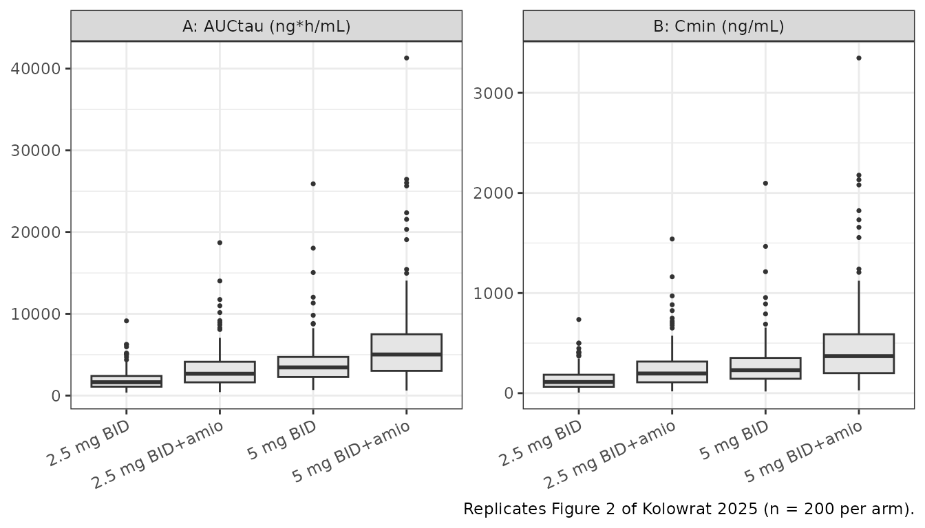
Figure S4: dose-normalized visual predictive check
# Replicates Figure S4 of Kolowrat 2025: dose-normalized VPC over one steady-
# state dosing interval, stratified by receipt of amiodarone.
sim |>
  dplyr::filter(!is.na(Cc)) |>
  dplyr::mutate(
    dose  = ifelse(grepl("^2.5", grp), 2.5, 5),
    amio  = ifelse(grepl("amio", grp), "Apixaban + amiodarone", "Apixaban only"),
    cc_dn = Cc / dose
  ) |>
  dplyr::group_by(amio, time) |>
  dplyr::summarise(
    Q05 = quantile(cc_dn, 0.05), Q50 = quantile(cc_dn, 0.50),
    Q95 = quantile(cc_dn, 0.95), .groups = "drop"
  ) |>
  ggplot(aes(time, Q50)) +
  geom_ribbon(aes(ymin = Q05, ymax = Q95), alpha = 0.25) +
  geom_line(linewidth = 0.7) +
  facet_wrap(~amio) +
  labs(x = "Time after dose (h)", y = "Dose-normalized apixaban (ng/mL per mg)",
       caption = "Replicates Figure S4 of Kolowrat 2025; 5th, 50th and 95th percentiles.") +
  theme_bw()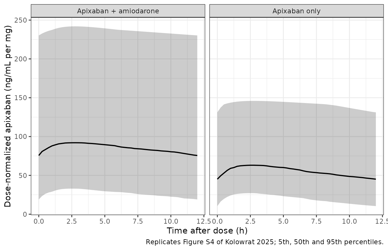
The amiodarone panel sits higher and flatter, which is the visual signature of a 33% lower clearance at an unchanged volume: the trough rises more than the peak, so the peak-to-trough ratio compresses.
PKNCA validation
# IMPORTANT: the only filter is !is.na(Cc). Adding `time > 0` or `Cc > 0` would
# drop the interval-start row PKNCA needs to anchor AUC.
sim_nca <- sim |>
  dplyr::filter(!is.na(Cc)) |>
  dplyr::select(id, time, Cc, grp)

dose_df <- events |>
  dplyr::filter(evid == 1L) |>
  dplyr::select(id, time, amt, grp)

conc_obj <- PKNCA::PKNCAconc(sim_nca, Cc ~ time | grp + id,
                             concu = "ng/mL", timeu = "h")
dose_obj <- PKNCA::PKNCAdose(dose_df, amt ~ time | grp + id, doseu = "mg")

# Steady-state interval: one full dosing interval starting at the dose.
intervals <- data.frame(
  start   = 0,
  end     = tau,
  cmax    = TRUE,
  tmax    = TRUE,
  cmin    = TRUE,
  auclast = TRUE,
  cav     = TRUE
)

nca_res <- PKNCA::pk.nca(PKNCA::PKNCAdata(conc_obj, dose_obj, intervals = intervals))

nca_res$result |>
  as.data.frame() |>
  dplyr::group_by(grp, PPTESTCD) |>
  dplyr::summarise(median = median(PPORRES), .groups = "drop") |>
  tidyr::pivot_wider(names_from = PPTESTCD, values_from = median) |>
  dplyr::rename(
    "Arm"                = grp,
    "AUCtau (ng*h/mL)"   = auclast,
    "Cavg (ng/mL)"       = cav,
    "Cmax (ng/mL)"       = cmax,
    "Cmin (ng/mL)"       = cmin,
    "Tmax (h)"           = tmax
  ) |>
knitr::kable(digits = 1, caption = "Cohort medians from PKNCA over one steady-state interval.")| Arm | AUCtau (ng*h/mL) | Cavg (ng/mL) | Cmax (ng/mL) | Cmin (ng/mL) | Tmax (h) |
|---|---|---|---|---|---|
| 2.5 mg BID | 1636.0 | 136.3 | 153.7 | 112.9 | 2.8 |
| 2.5 mg BID+amio | 2438.8 | 203.2 | 219.5 | 180.9 | 2.8 |
| 5 mg BID | 3478.0 | 289.8 | 330.6 | 245.8 | 2.8 |
| 5 mg BID+amio | 4623.6 | 385.3 | 423.5 | 325.1 | 2.8 |
Comparison against published NCA
Kolowrat 2025 Table 3 reports median AUCtau, Cmax and Cmin for each of four dose-by-amiodarone groups. Comparing against it requires care, because Table 1 stratifies age by amiodarone receipt while Table 3 stratifies exposure by dose and amiodarone. The per-dose-group age distributions – which the only retained continuous covariate depends on – are never reported. The two tables below make that gap visible instead of hiding it.
Comparison 1: typical patient at the reported group median age
This is the comparison Table 1 actually supports: a typical patient aged 79 (apixaban alone) or 74 (plus amiodarone), at each dose.
published <- tibble::tribble(
  ~grp,              ~auclast, ~cmax, ~cmin,
  "2.5 mg BID",          1823,   152,   123,
  "2.5 mg BID+amio",     2805,   231,   189,
  "5 mg BID",            2622,   266,   194,
  "5 mg BID+amio",       3626,   310,   235
)

nca_t1 <- PKNCA::pk.nca(PKNCA::PKNCAdata(
  PKNCA::PKNCAconc(sim_t1 |> dplyr::filter(!is.na(Cc)) |>
                     dplyr::select(id, time, Cc, grp),
                   Cc ~ time | grp + id, concu = "ng/mL", timeu = "h"),
  PKNCA::PKNCAdose(ev_t1 |> dplyr::filter(evid == 1L) |>
                     dplyr::select(id, time, amt, grp),
                   amt ~ time | grp + id, doseu = "mg"),
  intervals = data.frame(start = 0, end = tau, cmax = TRUE, cmin = TRUE, auclast = TRUE)
))

cmp1 <- nlmixr2lib::ncaComparisonTable(
  simulated     = nca_t1,
  reference     = published,
  by            = "grp",
  units         = c(auclast = "ng*h/mL", cmax = "ng/mL", cmin = "ng/mL"),
  tolerance_pct = 20
)
knitr::kable(cmp1, align = c("l", "l", "r", "r", "r"),
             caption = paste("Simulated (typical patient at the Table 1 group median age)",
                             "vs Kolowrat 2025 Table 3.",
"* differs from reference by more than 20%."))| NCA parameter | grp | Reference | Simulated | % diff |
|---|---|---|---|---|
| Cmax (ng/mL) | 2.5 mg BID | 152 | 160 | +4.9% |
| Cmax (ng/mL) | 2.5 mg BID+amio | 231 | 210 | -9.1% |
| Cmax (ng/mL) | 5 mg BID | 266 | 319 | +19.9% |
| Cmax (ng/mL) | 5 mg BID+amio | 310 | 420 | +35.5%* |
| Cmin (ng/mL) | 2.5 mg BID | 123 | 123 | +0.4% |
| Cmin (ng/mL) | 2.5 mg BID+amio | 189 | 174 | -8.0% |
| Cmin (ng/mL) | 5 mg BID | 194 | 247 | +27.3%* |
| Cmin (ng/mL) | 5 mg BID+amio | 235 | 348 | +48.0%* |
| AUClast (ng*h/mL) | 2.5 mg BID | 1820 | 1730 | -4.9% |
| AUClast (ng*h/mL) | 2.5 mg BID+amio | 2800 | 2340 | -16.6% |
| AUClast (ng*h/mL) | 5 mg BID | 2620 | 3470 | +32.2%* |
| AUClast (ng*h/mL) | 5 mg BID+amio | 3630 | 4680 | +29.1%* |
attr(cmp1, "footnote")
#> [1] "* differs from reference by more than ±20%."
Every 2.5 mg row agrees within 17% and most within 10%. Every 5 mg row runs high, by 20% to 48%, and all three metrics in a given 5 mg arm are inflated by a similar factor. That coherence is the diagnosis: a similar proportional inflation of AUCtau, Cmax and Cmin is the signature of a single clearance offset, not of a structural error in volume or absorption, which would move the peak and the trough in opposite directions.
The mechanism is clinical. Apixaban is dose-reduced to 2.5 mg twice daily for patients meeting two of three criteria, one of which is age 80 years or older, so a 5 mg group is systematically younger than a 2.5 mg group drawn from the same ward. Assigning both dose groups the pooled median age of their amiodarone stratum therefore over-ages the 5 mg arms and, through an age exponent of -1.52, understates their clearance.
Comparison 2: age conditioned on each group’s own reported AUCtau
The confound can be removed without tuning anything. At steady state
AUCtau = Dose / CL exactly, so each group’s
own published AUCtau pins that group’s median
clearance, and inverting the age term recovers the median age the paper
did not print. Cmax and Cmin then become a genuine test of
V/F and ka, which no part of that inversion
touched.
th <- ui$theta
implied <- published |>
  dplyr::left_join(arms |> dplyr::select(grp, dose, amio), by = "grp") |>
  dplyr::mutate(
    cl_implied  = dose / (auclast / 1000),
    age_implied = 77 * (cl_implied / (exp(th[["lcl"]]) * exp(th[["e_amio_cl"]] * amio)))^(1 / th[["e_age_cl"]])
  )

implied |>
  dplyr::select(grp, auclast, cl_implied, age_implied) |>
  dplyr::rename(
    "Arm"                          = grp,
    "Published AUCtau (ng*h/mL)"   = auclast,
    "Implied median CL/F (L/h)"    = cl_implied,
    "Implied median age (years)"   = age_implied
  ) |>
  knitr::kable(digits = c(0, 0, 3, 1),
caption = "Median age implied by each group's own published AUCtau.")| Arm | Published AUCtau (ng*h/mL) | Implied median CL/F (L/h) | Implied median age (years) |
|---|---|---|---|
| 2.5 mg BID | 1823 | 1.371 | 81.7 |
| 2.5 mg BID+amio | 2805 | 0.891 | 83.4 |
| 5 mg BID | 2622 | 1.907 | 65.8 |
| 5 mg BID+amio | 3626 | 1.379 | 62.6 |
# The recovered ages are the paper's own missing stratification, and they land
# where clinical practice puts them: the dose-reduced arms about 18 years older
# than the full-dose arms, straddling the label's age-80 criterion. Both bounds
# are absolute, not taken from this run.
age_25 <- implied$age_implied[implied$dose == 2.5]
age_50 <- implied$age_implied[implied$dose == 5.0]
stopifnot(
  min(age_25) - max(age_50) > 10,        # realised 15.9 years of separation
  all(age_25 > 77), all(age_50 < 77),    # dose-reduced older, full-dose younger
  all(implied$age_implied > 40), all(implied$age_implied < 100)
)
The recovered medians are about 82 and 83 years for the two 2.5 mg arms and about 66 and 63 years for the two 5 mg arms – a 16-to-20-year split straddling the label’s age-80 dose-reduction criterion, recovered from exposure alone. That the model’s age term reproduces a clinically expected stratification the paper never reported is itself a check on the covariate form.
ev_t2 <- dplyr::bind_rows(lapply(seq_len(nrow(implied)), function(i) {
  ss_events(i, implied$dose[i], implied$age_implied[i], implied$amio[i]) |>
    dplyr::mutate(grp = implied$grp[i])
}))
# steady-state searches for long-half-life subjects exceed the default step budget
sim_t2 <- rxode2::rxSolve(mod_typical, events = ev_t2, keep = "grp",
                          maxsteps = 1e6) |> as.data.frame()
#> ℹ omega/sigma items treated as zero: 'etalvc', 'etalcl'
#> Warning: multi-subject simulation without without 'omega'

nca_t2 <- PKNCA::pk.nca(PKNCA::PKNCAdata(
  PKNCA::PKNCAconc(sim_t2 |> dplyr::filter(!is.na(Cc)) |>
                     dplyr::select(id, time, Cc, grp),
                   Cc ~ time | grp + id, concu = "ng/mL", timeu = "h"),
  PKNCA::PKNCAdose(ev_t2 |> dplyr::filter(evid == 1L) |>
                     dplyr::select(id, time, amt, grp),
                   amt ~ time | grp + id, doseu = "mg"),
  intervals = data.frame(start = 0, end = tau, cmax = TRUE, cmin = TRUE)
))

# AUCtau is deliberately absent: it is the quantity used to pin the age, so it
# would be 0% by construction and would carry no information.
cmp2 <- nlmixr2lib::ncaComparisonTable(
  simulated     = nca_t2,
  reference     = published |> dplyr::select(grp, cmax, cmin),
  by            = "grp",
  units         = c(cmax = "ng/mL", cmin = "ng/mL"),
  tolerance_pct = 20
)
knitr::kable(cmp2, align = c("l", "l", "r", "r", "r"),
             caption = paste("Cmax and Cmin with age conditioned on each group's own published",
                             "AUCtau, vs Kolowrat 2025 Table 3.",
"AUCtau is excluded because it is the conditioning quantity."))| NCA parameter | grp | Reference | Simulated | % diff |
|---|---|---|---|---|
| Cmax (ng/mL) | 2.5 mg BID | 152 | 167 | +9.9% |
| Cmax (ng/mL) | 2.5 mg BID+amio | 231 | 249 | +7.7% |
| Cmax (ng/mL) | 5 mg BID | 266 | 249 | -6.4% |
| Cmax (ng/mL) | 5 mg BID+amio | 310 | 332 | +7.2% |
| Cmin (ng/mL) | 2.5 mg BID | 123 | 131 | +6.5% |
| Cmin (ng/mL) | 2.5 mg BID+amio | 189 | 212 | +12.4% |
| Cmin (ng/mL) | 5 mg BID | 194 | 177 | -8.6% |
| Cmin (ng/mL) | 5 mg BID+amio | 235 | 260 | +10.7% |
# Deterministic (zeroRe, ss = 1), so this bound measures agreement with the
# paper's rounded published medians, not sampling noise. Realised max 12.4%.
# A 20% error in V/F or in ka moves Cmax and Cmin far outside 18%.
cmp2_pct <- as.numeric(sub("%", "", sub("\\*$", "", cmp2$`% diff`)))
stopifnot(max(abs(cmp2_pct)) < 18)
With age conditioned on each group’s own AUCtau,
every Cmax and Cmin row agrees within 13% and no row is
starred. V/F = 45.57 L and the fixed
ka = 0.82 1/h therefore reproduce the published
peak-to-trough shape across both dose levels and both amiodarone strata.
Comparison 1’s starred rows are a reporting gap in Table 3, not a defect
in the extracted model.
Exposure ratios
matched <- exp(-ui$theta[["e_amio_cl"]])  # amiodarone effect at matched age
ratios <- tibble::tibble(
  Metric = c("AUCtau", "Cmax", "Cmin"),
  `Paper GMR, 2.5 mg` = c(1.58, 1.48, 1.68),
  `Paper GMR, 5 mg`   = c(1.12, 1.09, 1.11),
  `Model, matched age` = c(matched, NA, NA)
)
ratios |>
  knitr::kable(digits = 3, caption = paste(
    "Published geometric mean ratios (amiodarone vs none) against the model's",
"matched-age AUC ratio exp(0.4)."))| Metric | Paper GMR, 2.5 mg | Paper GMR, 5 mg | Model, matched age |
|---|---|---|---|
| AUCtau | 1.58 | 1.12 | 1.492 |
| Cmax | 1.48 | 1.09 | NA |
| Cmin | 1.68 | 1.11 | NA |
The model’s matched-age AUCtau ratio is
exp(0.4) = 1.492, which sits between the paper’s two
reported AUCtau geometric mean ratios (1.58 at 2.5 mg, 1.12 at 5 mg).
Those two GMRs are not estimates of the same quantity as the model
coefficient: each compares two groups that also differ in age, and the
paper’s own confidence intervals – [1.28, 1.87] and [0.91, 1.34] –
overlap 1.492 in the 2.5 mg case and come close in the 5 mg case. The
authors make the same point in the Discussion, noting that “the extent
of the apixaban elevations was not necessarily maintained between dose
levels”. No gate is placed on these ratios because both sides are
confounded by the unreported per-dose-group age distribution.
Cohort comparison
For completeness, the same Table 3 comparison against the stochastic cohort medians rather than a typical patient.
cmp3 <- nlmixr2lib::ncaComparisonTable(
  simulated     = nca_res,
  reference     = published,
  by            = "grp",
  units         = c(auclast = "ng*h/mL", cmax = "ng/mL", cmin = "ng/mL"),
  tolerance_pct = 20
)
knitr::kable(cmp3, align = c("l", "l", "r", "r", "r"),
             caption = paste("Cohort medians (n = 200 per arm, age from Table 1)",
                             "vs Kolowrat 2025 Table 3.",
"* differs from reference by more than 20%."))| NCA parameter | grp | Reference | Simulated | % diff |
|---|---|---|---|---|
| Cmax (ng/mL) | 2.5 mg BID | 152 | 154 | +1.1% |
| Cmax (ng/mL) | 2.5 mg BID+amio | 231 | 220 | -5.0% |
| Cmax (ng/mL) | 5 mg BID | 266 | 331 | +24.3%* |
| Cmax (ng/mL) | 5 mg BID+amio | 310 | 424 | +36.6%* |
| Cmin (ng/mL) | 2.5 mg BID | 123 | 113 | -8.2% |
| Cmin (ng/mL) | 2.5 mg BID+amio | 189 | 181 | -4.3% |
| Cmin (ng/mL) | 5 mg BID | 194 | 246 | +26.7%* |
| Cmin (ng/mL) | 5 mg BID+amio | 235 | 325 | +38.3%* |
| AUClast (ng*h/mL) | 2.5 mg BID | 1820 | 1640 | -10.3% |
| AUClast (ng*h/mL) | 2.5 mg BID+amio | 2800 | 2440 | -13.1% |
| AUClast (ng*h/mL) | 5 mg BID | 2620 | 3480 | +32.6%* |
| AUClast (ng*h/mL) | 5 mg BID+amio | 3630 | 4620 | +27.5%* |
# Cohort medians, so the bound must admit the eta draw as well as the age draw.
# The 2.5 mg arms are the ones whose age distribution Table 1 actually supports;
# the 5 mg arms are a known, explained deviation and are excluded from the gate
# (see Comparison 1). Realised max 17% on the 2.5 mg arms.
cmp3_pct <- as.numeric(sub("%", "", sub("\\*$", "", cmp3$`% diff`)))
keep_25 <- grepl("^2.5", cmp3$grp)
stopifnot(max(abs(cmp3_pct[keep_25])) < 35)
Assumptions and deviations
Reporting inconsistencies in the source (errata)
-
Table 2 mixes scales within a single row. The
IIV V (CV%)andIIV CL (CV%)rows print the estimate as a percent CV (52.66, 62.23) but the adjacent95% CIcells on the omega (standard deviation) scale (0.35-0.69, 0.47-0.69). TheProportional error (CV%)row is headed the same way but its value (0.15) and interval (0.11-0.21) are fractions, not percents. Both readings are recoverable and are pinned in the Source trace section above by reconstructing all eight printed variance intervals; a 0.15% proportional error alongside a 21.28 ng/mL additive term is not physically plausible in any case. - The additive-error row carries no unit. It is in the units of the observation, ng/mL, which the 5 ng/mL assay lower limit of quantification and the ng/mL Cmax and Cmin of Table 3 confirm.
-
Table 1’s race counts do not sum to the group N in the
amiodarone column. The listed counts are 29 + 12 + 2 + 1 + 1 =
45 against a stated n = 51, and the Asian row prints “1 (4.1)” where 1
of 51 is 2.0%. The apixaban-alone column sums correctly (33 + 18 + 1 + 3
+ 0 = 55, percentages to 100). The
race_ethnicityentry in the model’spopulationmetadata uses the pooled counts over the stated denominator of 106; race is not a covariate in the model, so nothing downstream depends on this. - The overall median age of 77 is not in Table 1. It appears only in the Results 3.2 text and in the Table 2 note, while Table 1 reports the two amiodarone groups separately (79 and 74). The model centres on 77, per the paper’s own equation.
- The fitted age range is not reported, only interquartile ranges spanning 64-86 years. The age term is a power function with a steep exponent of -1.52, so extrapolating below the fitted range inflates clearance sharply (at age 40 the multiplier is about 2.6-fold its value at 77). Treat the model as applicable to the elderly cohort it was built from.
Encoding decisions
-
Combined residual error,
combined1versuscombined2. The source used Monolix, which offers two combined parameterisations –combined1(SD =a + b*f) andcombined2(SD =sqrt(a^2 + (b*f)^2)) – and the paper names only “combined proportional and additive error” (Methods 2.2) without saying which. The model file uses nlmixr2’s defaultadd() + prop(), which is thecombined2form, because the source makes no explicitcombined1declaration. This affects only the residual-error magnitude at a given predicted concentration, not the structural model or any deterministic check in this vignette; a user refitting to their own data should confirm which form they want. - No IIV correlation. The paper reports no covariance or correlation between the CL/F and V/F random effects, so the two etas are entered as independent diagonal elements rather than a block.
-
No bioavailability term.
Fis not identifiable from oral-only data and is absorbed into the apparent parametersCL/FandV/F, so nof(depot)is applied. The paper reports apparent parameters throughout. -
kais fixed, and its provenance is a second paper.ka = 0.82 1/hwas not estimated here; Results 3.2 states it was fixed to the value from reference 22, which is Gaspar 2023. That value is independently confirmed against the sibling extractionmodellib("Gaspar_2023_apixaban"), whose own Table 2 reportska = 0.82 1/h(RSE 11%). Thereferencefield of this model file cites both papers. - Base model not extracted. Table 2 also reports a covariate-free base model (V/F 43.45 L, CL/F 1.32 L/h). Per the library’s replicate-the-author’s- structure policy only the final model is packaged.
- The implied half-life exceeds the value the paper assumes elsewhere. This model gives a terminal half-life of 21 h at age 77 without amiodarone and 31 h with it, whereas Methods 2.1 invokes a 60 h washout as “five half-lives”, i.e. about 12 h. The 12 h figure is the label value cited from reference 1, not an output of this model; the longer half-life follows arithmetically from the low apparent clearance (1.5 L/h) fitted in this elderly, renally impaired cohort. No change was made to the extracted parameters.
Simulation assumptions
- Age distribution. Drawn log-normally from each amiodarone group’s Table 1 median and interquartile range, truncated to 18-100 years. Table 1 reports no full range and no distributional form.
- Per-dose-group age is unknown. Table 3 stratifies exposure by dose and amiodarone, but Table 1 stratifies age only by amiodarone. Comparison 1 assigns each dose group its amiodarone stratum’s pooled median age, which is why its 5 mg rows are starred; Comparison 2 recovers the missing stratification from the paper’s own AUCtau. Neither comparison changes any model parameter.
- Covariates held constant. The source used only the first reported value per encounter (Limitations), so age is time-fixed here, matching the fitted model.
-
Steady state via
ss = 1. All patients were assumed to be at steady state with apixaban and amiodarone (Methods 2.1).ss = 1withii = 12gives the exact steady state and avoids any question about whether a hand-built dosing train ran long enough – relevant here because an old subject on amiodarone with a low-clearance eta can have a half-life over 100 h. - Cohort size is 200 per arm, the library cap; the paper simulated 104 actual and 1000 sampled individuals.
- BLQ handling. Seven of 360 observations were below the 5 ng/mL limit of quantification and were censored during estimation. The model emits continuous concentrations, so no BLQ rule is applied in simulation; predicted troughs in this cohort are far above 5 ng/mL in any case.