Zonisamide (Hashimoto 1994)
Source:vignettes/articles/Hashimoto_1994_zonisamide.Rmd
Hashimoto_1994_zonisamide.RmdModel and source
- Citation: Hashimoto Y, Odani A, Tanigawara Y, Yasuhara M, Okuno T, Hori R. Population analysis of the dose-dependent pharmacokinetics of zonisamide in epileptic patients. Biol Pharm Bull. 1994;17(2):323-326. doi:10.1248/bpb.17.323
- Description: Steady-state Michaelis-Menten population PK model for zonisamide in 68 Japanese epileptic patients (pediatric + adult) on chronic oral zonisamide. A power-of-weight body-size factor scales both volume of distribution and Vmax; concomitant carbamazepine multiplicatively increases Vmax (Hashimoto 1994 Eqs. 1-4).
- Article: Biol Pharm Bull 17(2):323-326 (1994)
Population
Hashimoto 1994 (Table I) collected steady-state therapeutic-drug-monitoring (TDM) data from 68 Japanese epileptic patients (60 outpatients, 31 female, mean age 11.2 +/- 6.4 years, mean body weight 33.4 +/- 17.7 kg) at Kyoto University Hospital between November 1989 and July 1992. Thirty patients were under 10 years old; 5 were over 20. Mean daily zonisamide dose was 135 +/- 104 mg, administered orally as Excegran tablet or powder (Dainippon Pharmaceutical Co., Osaka) at 12-hour intervals to 62 of 68 patients. Two hundred sixty-six serum samples were collected at steady state (>= 1 month of stable therapy): 208 samples 2-6 h post-dose for approximate peak levels, 33 samples at the 12-h trough. Only 2 of 68 patients were on zonisamide monotherapy; 37 received concomitant carbamazepine, 32 valproate, 27 phenytoin, and 5 phenobarbital.
The same information is available programmatically via the model’s
population metadata
(readModelDb("Hashimoto_1994_zonisamide")$population).
Source trace
The per-parameter origin is recorded as an in-file comment next to
each ini() entry in
inst/modeldb/specificDrugs/Hashimoto_1994_zonisamide.R. The
table below collects them in one place for review.
| Equation / parameter | Value | Source location |
|---|---|---|
Cc = central / vc |
n/a | Eq. 1, page 324 (steady-state form) |
SIZE_i = 33 * (WT/33)^theta1 |
n/a | Eq. 2, page 324 |
vc = exp(lvc) * (WT/33)^theta1 |
n/a | Eq. 3, page 324 |
vmax = exp(lvmax) * SIZE * theta2^CBZ |
n/a | Eq. 4 rearrangement, page 324 |
d/dt(central) = -vmax * Cc / (km + Cc) |
n/a | Michaelis-Menten form implied by Eq. 4 |
Cc ~ prop(propSd) |
n/a | Eq. 5, page 324 |
V (typical Vc at 33 kg) |
1.27 L/kg | Table II, page 325; 1.27 * 33 = 41.91 L |
Vmax (typical at 33 kg) |
27.6 mg/d/kg | Table II; 27.6 * 33 = 910.8 mg/d |
Km |
45.9 mg/L | Table II, page 325 (45.9 ug/mL) |
theta1 (e_wt_vc_vmax) |
0.741 | Table II, page 325 (95% CI 0.665-0.817) |
theta2 (e_conmed_cbz_vmax) |
1.13 | Table II, page 325 (95% CI 1.02-1.24) |
omega_CL -> etalvmax variance |
0.297^2 = 0.0882 | Table II (omega_CL = 29.7 % CV) |
sigma (propSd) |
0.178 | Table II, page 325 (95% CI 14.5-20.7 %) |
Virtual cohort
Original observed data are not publicly available. The cohort below approximates the published trial demographics (Hashimoto 1994 Table I) and the dose-grid structure of Figure 4 (page 326): two reference body weights (33 kg adult-typical and 10 kg pediatric-typical), four daily-dose levels (2.5, 5, 10, 20 mg/d/kg), and a binary CBZ coadministration indicator. Each combination is replicated by 40 simulated subjects to capture the omega_CL = 29.7 % between-subject variability translated to log-normal IIV on Vmax (see Assumptions and deviations).
set.seed(20251010L)

# Hashimoto 1994 Methods: tau = 12 h = 0.5 day; daily dose split 1:1 across
# two daily administrations. Vmax in mg/day requires time in days.
tau           <- 0.5                                 # dosing interval (day)
days_to_ss    <- 30                                  # > 10 half-lives at typical conc
dose_times    <- seq(0, days_to_ss - tau, by = tau)  # dose at every tau
obs_window    <- seq(days_to_ss - tau, days_to_ss, length.out = 51)  # last interval

# Figure 4 dose grid: 2.5, 5, 10, 20 mg/d/kg, both reference weights, no CBZ.
fig4_grid <- expand.grid(
  WT_kg         = c(10, 33),
  daily_mgkg    = c(2.5, 5, 10, 20),
  CONMED_CBZ    = c(0, 1),
  stringsAsFactors = FALSE
) |>
  dplyr::mutate(
    per_dose_mg  = daily_mgkg * WT_kg / 2,           # split daily dose across 2 administrations
    treatment    = sprintf("%d kg / %g mg/d/kg / CBZ=%d", WT_kg, daily_mgkg, CONMED_CBZ)
  )

n_per_group <- 40L

make_cohort <- function(per_dose_mg, WT_kg, CONMED_CBZ, treatment,
                        n, id_offset) {
  ids <- id_offset + seq_len(n)
  # Build dose rows and observation rows separately so a time that appears
  # in both (e.g. the final dose at 29.5 d also being the first observation)
  # does NOT collapse - we want two distinct rows differing only on evid.
  dose_rows <- expand.grid(id = ids, time = dose_times, KEEP.OUT.ATTRS = FALSE)
  dose_rows$evid <- 1L
  dose_rows$amt  <- per_dose_mg
  dose_rows$cmt  <- "central"
  obs_rows <- expand.grid(id = ids, time = obs_window, KEEP.OUT.ATTRS = FALSE)
  obs_rows$evid <- 0L
  obs_rows$amt  <- 0
  obs_rows$cmt  <- NA_character_
  rows <- rbind(dose_rows, obs_rows)
  rows$WT         <- WT_kg
  rows$CONMED_CBZ <- CONMED_CBZ
  rows$treatment  <- treatment
  rows[order(rows$id, rows$time, -rows$evid), ]
}

events <- do.call(
  dplyr::bind_rows,
  lapply(seq_len(nrow(fig4_grid)), function(i) {
    g <- fig4_grid[i, ]
    make_cohort(
      per_dose_mg = g$per_dose_mg, WT_kg = g$WT_kg,
      CONMED_CBZ = g$CONMED_CBZ, treatment = g$treatment,
      n = n_per_group, id_offset = (i - 1L) * n_per_group
    )
  })
)

# Sanity guard: every (id, time, evid) row must be unique - duplicate ids
# across cohorts would otherwise silently merge into Frankenstein subjects.
stopifnot(!anyDuplicated(events[, c("id", "time", "evid")]))
Simulation
mod <- readModelDb("Hashimoto_1994_zonisamide")
sim <- rxode2::rxSolve(
  mod, events = events,
  keep = c("treatment", "WT", "CONMED_CBZ"),
  returnType = "data.frame"
)
#> ℹ parameter labels from comments will be replaced by 'label()'
For deterministic (typical-value) replication of Figure 4 - where the paper sets eta_CL = 0 - zero out the random effects:
mod_typical <- mod |> rxode2::zeroRe()
#> ℹ parameter labels from comments will be replaced by 'label()'
sim_typical <- rxode2::rxSolve(
  mod_typical, events = events,
  keep = c("treatment", "WT", "CONMED_CBZ"),
  returnType = "data.frame"
)
#> ℹ omega/sigma items treated as zero: 'etalvmax'
#> Warning: multi-subject simulation without without 'omega'
Replicate published figures
Figure 4 - predicted steady-state serum zonisamide
Hashimoto 1994 Figure 4 shows the predicted serum zonisamide concentration over one 12-h dosing interval at steady state, for a typical 33-kg patient (panel a) and a typical 10-kg patient (panel b), at four daily-dose levels (2.5, 5, 10, 20 mg/d/kg), with (dotted) and without (solid) concomitant carbamazepine. The paper states “The dotted (with carbamazepine) and solid (without carbamazepine) lines are drawn using Eqs. 1-4 and the parameter value listed in Table II, assuming that eta_CL is equal to zero” (Figure 4 caption, page 326).
sim_typical |>
  dplyr::filter(time >= days_to_ss - tau) |>
  dplyr::mutate(
    time_h  = (time - (days_to_ss - tau)) * 24,
    WT_lab  = factor(paste0(WT, " kg patient"),
                     levels = c("10 kg patient", "33 kg patient")),
    daily_mgkg = factor(
      vapply(treatment, function(t) strsplit(t, " / ")[[1]][2], character(1)),
      levels = c("2.5 mg/d/kg", "5 mg/d/kg", "10 mg/d/kg", "20 mg/d/kg")
    ),
    CBZ_lab = ifelse(CONMED_CBZ == 1, "with CBZ", "without CBZ")
  ) |>
  ggplot(aes(time_h, Cc, colour = daily_mgkg, linetype = CBZ_lab)) +
  geom_line(linewidth = 0.7) +
  facet_wrap(~WT_lab) +
  scale_y_log10(limits = c(1, 100), breaks = c(1, 10, 100)) +
  scale_x_continuous(breaks = c(2, 6, 12)) +
  labs(
    x = "Time after dose (h)", y = "Serum zonisamide conc. (mg/L)",
    colour = "Daily dose", linetype = NULL,
    title = "Figure 4 - predicted steady-state zonisamide (12-h interval)",
    caption = "Replicates Figure 4 of Hashimoto 1994 (page 326)."
  )
#> Warning: Removed 480 rows containing missing values or values outside the scale range
#> (`geom_line()`).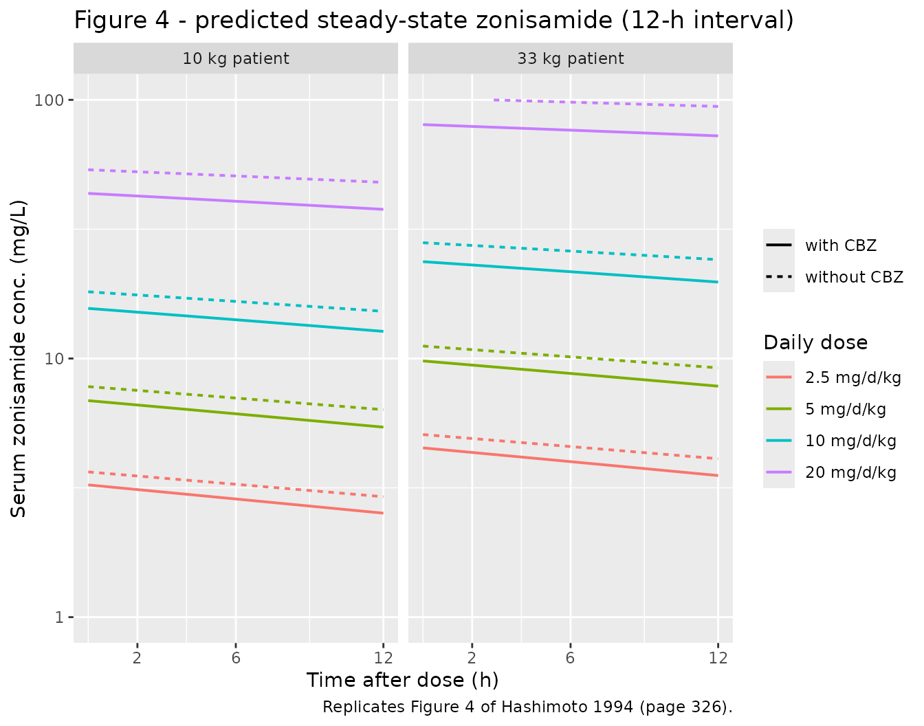
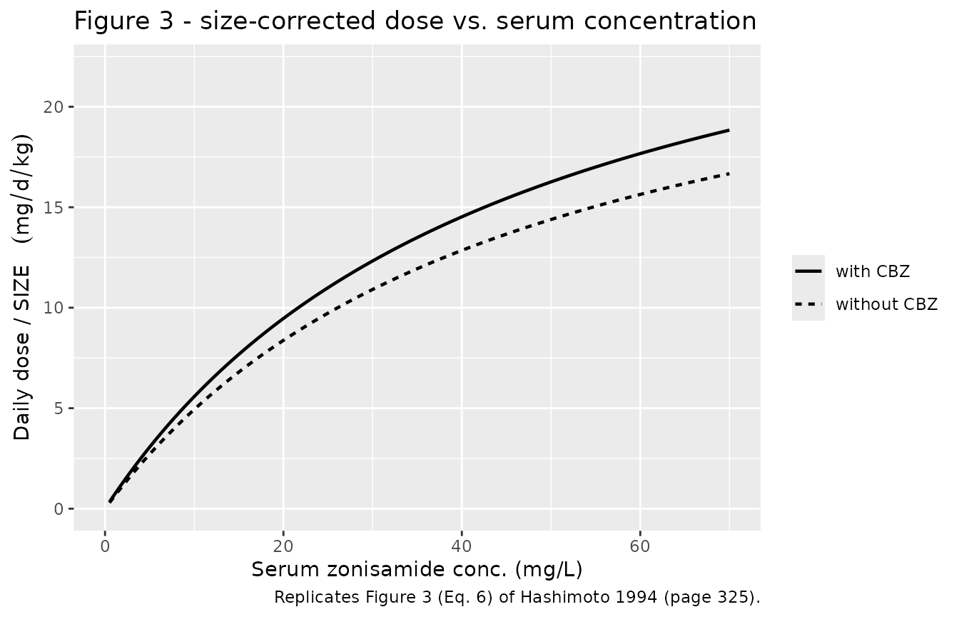
Figure 3 - size-corrected dose vs. steady-state concentration with vs. without CBZ
Hashimoto 1994 Figure 3 plots size-corrected daily dose
(D / SIZE, with SIZE = 33 * (WT/33)^0.741) against
steady-state serum concentration, stratified by concomitant
carbamazepine status. The least-squares fit at the population mean
parameters uses Eq. 6 (page 325):
D/SIZE = Vmax * SZC / (Km + SZC),
with Vmax replaced by Vmax * theta2^CBZ for the CBZ stratum. Below we sweep SZC and plot the implied D/SIZE for both strata; the model file’s typical values reproduce this curve exactly.
szc_grid <- seq(0.5, 70, length.out = 200)
vmax_typ <- 27.6   # mg/d/kg, Table II
km_typ   <- 45.9   # mg/L,    Table II
theta2   <- 1.13   # Table II

mm_fits <- tibble::tibble(
  szc = rep(szc_grid, 2),
  CBZ = rep(c("without CBZ", "with CBZ"), each = length(szc_grid)),
  vmax_eff = ifelse(CBZ == "with CBZ", vmax_typ * theta2, vmax_typ),
  d_per_size = vmax_eff * szc / (km_typ + szc)
)

ggplot(mm_fits, aes(szc, d_per_size, linetype = CBZ)) +
  geom_line(linewidth = 0.8) +
  scale_y_continuous(limits = c(0, 22)) +
  scale_x_continuous(limits = c(0, 70)) +
  labs(
    x = "Serum zonisamide conc. (mg/L)",
    y = expression("Daily dose / SIZE   "(mg/d/kg)),
    linetype = NULL,
    title = "Figure 3 - size-corrected dose vs. serum concentration",
    caption = "Replicates Figure 3 (Eq. 6) of Hashimoto 1994 (page 325)."
  )
PKNCA validation
Steady-state NCA is performed on the final dosing interval (day 29.5 -> 30). For multiple-dose steady-state we report Cmax,ss, Cmin (Ctau), Cavg, and AUC0-tau within each treatment group.
sim_nca <- sim |>
  dplyr::filter(time >= days_to_ss - tau & !is.na(Cc)) |>
  dplyr::select(id, time, Cc, treatment) |>
  as.data.frame()

dose_df <- events |>
  dplyr::filter(evid == 1L & time >= days_to_ss - tau) |>
  dplyr::select(id, time, amt, treatment) |>
  as.data.frame()

conc_obj <- PKNCA::PKNCAconc(sim_nca, Cc ~ time | treatment + id,
                             concu = "mg/L", timeu = "day")
dose_obj <- PKNCA::PKNCAdose(dose_df, amt ~ time | treatment + id,
                             doseu = "mg")

start_ss <- days_to_ss - tau
end_ss   <- days_to_ss

intervals <- data.frame(
  start    = start_ss,
  end      = end_ss,
  cmax     = TRUE,
  cmin     = TRUE,
  tmax     = TRUE,
  auclast  = TRUE,
  cav      = TRUE
)

nca_res <- PKNCA::pk.nca(PKNCA::PKNCAdata(conc_obj, dose_obj, intervals = intervals))
nca_summary <- summary(nca_res)
knitr::kable(nca_summary, caption = "Steady-state NCA over the final 12-h dosing interval, by treatment group.")| Interval Start | Interval End | treatment | N | AUClast (day*mg/L) | Cmax (mg/L) | Cmin (mg/L) | Tmax (day) | Cav (mg/L) |
|---|---|---|---|---|---|---|---|---|
| 29.5 | 30 | 10 kg / 10 mg/d/kg / CBZ=0 | 40 | 8.38 [40.4] | 18.4 [36.5] | 15.2 [44.8] | 0.000 [0.000, 0.000] | 16.8 [40.4] |
| 29.5 | 30 | 10 kg / 10 mg/d/kg / CBZ=1 | 40 | 6.92 [29.2] | 15.4 [26.2] | 12.4 [32.5] | 0.000 [0.000, 0.000] | 13.8 [29.2] |
| 29.5 | 30 | 10 kg / 2.5 mg/d/kg / CBZ=0 | 40 | 1.61 [31.2] | 3.61 [27.7] | 2.85 [35.0] | 0.000 [0.000, 0.000] | 3.22 [31.2] |
| 29.5 | 30 | 10 kg / 2.5 mg/d/kg / CBZ=1 | 40 | 1.31 [30.4] | 3.02 [26.0] | 2.26 [35.4] | 0.000 [0.000, 0.000] | 2.62 [30.4] |
| 29.5 | 30 | 10 kg / 20 mg/d/kg / CBZ=0 | 40 | 24.4 [49.6] | 52.0 [46.1] | 45.7 [53.5] | 0.000 [0.000, 0.000] | 48.8 [49.6] |
| 29.5 | 30 | 10 kg / 20 mg/d/kg / CBZ=1 | 40 | 18.8 [53.1] | 40.9 [48.3] | 34.5 [58.7] | 0.000 [0.000, 0.000] | 37.7 [53.1] |
| 29.5 | 30 | 10 kg / 5 mg/d/kg / CBZ=0 | 40 | 3.63 [38.5] | 8.05 [34.3] | 6.51 [43.2] | 0.000 [0.000, 0.000] | 7.26 [38.5] |
| 29.5 | 30 | 10 kg / 5 mg/d/kg / CBZ=1 | 40 | 3.37 [44.9] | 7.56 [39.0] | 5.97 [51.8] | 0.000 [0.000, 0.000] | 6.75 [44.9] |
| 29.5 | 30 | 33 kg / 10 mg/d/kg / CBZ=0 | 40 | 14.1 [34.6] | 30.3 [32.1] | 26.1 [37.4] | 0.000 [0.000, 0.000] | 28.2 [34.6] |
| 29.5 | 30 | 33 kg / 10 mg/d/kg / CBZ=1 | 40 | 11.6 [45.7] | 25.4 [41.4] | 21.1 [50.5] | 0.000 [0.000, 0.000] | 23.2 [45.7] |
| 29.5 | 30 | 33 kg / 2.5 mg/d/kg / CBZ=0 | 40 | 2.35 [33.1] | 5.24 [29.1] | 4.20 [37.7] | 0.000 [0.000, 0.000] | 4.70 [33.1] |
| 29.5 | 30 | 33 kg / 2.5 mg/d/kg / CBZ=1 | 40 | 2.04 [30.9] | 4.61 [27.5] | 3.59 [34.7] | 0.000 [0.000, 0.000] | 4.08 [30.9] |
| 29.5 | 30 | 33 kg / 20 mg/d/kg / CBZ=0 | 40 | 52.8 [57.6] | 110 [54.4] | 101 [61.1] | 0.000 [0.000, 0.000] | 106 [57.6] |
| 29.5 | 30 | 33 kg / 20 mg/d/kg / CBZ=1 | 40 | 38.5 [59.6] | 81.4 [55.3] | 72.6 [64.4] | 0.000 [0.000, 0.000] | 77.0 [59.6] |
| 29.5 | 30 | 33 kg / 5 mg/d/kg / CBZ=0 | 40 | 5.16 [35.0] | 11.4 [31.6] | 9.31 [38.7] | 0.000 [0.000, 0.000] | 10.3 [35.0] |
| 29.5 | 30 | 33 kg / 5 mg/d/kg / CBZ=1 | 40 | 4.32 [40.1] | 9.73 [35.7] | 7.62 [45.2] | 0.000 [0.000, 0.000] | 8.64 [40.1] |
Comparison against the paper’s Eq. 6 prediction
Hashimoto 1994 does not tabulate Cmax,ss / Cmin,ss / AUC0-tau by dose
group; the validation reference is the predicted typical-value
steady-state curve in Figure 4 (replicated above) plus the algebraic
relation in Eq. 6 (D/SIZE = Vmax \* SZC / (Km + SZC)). The
table below confirms that the simulated average steady-state
concentration (Cavg,sim) agrees with the analytical Eq. 6
prediction (Cavg,Eq6) for each combination of body weight,
daily dose, and CBZ status (typical-value simulation, no IIV).
cavg_sim <- sim_typical |>
  dplyr::filter(time >= days_to_ss - tau) |>
  dplyr::group_by(treatment, WT, CONMED_CBZ) |>
  dplyr::summarise(Cavg_sim = mean(Cc), .groups = "drop")

eq6_pred <- fig4_grid |>
  dplyr::mutate(
    size_i   = 33 * (WT_kg / 33)^0.741,
    vmax_eff = vmax_typ * size_i * theta2^CONMED_CBZ,
    d_rate   = daily_mgkg * WT_kg,                       # mg/day at the patient level
    # Solve D = Vmax_eff * SZC / (Km + SZC) -> SZC = D*Km / (Vmax_eff - D)
    Cavg_Eq6 = ifelse(vmax_eff > d_rate,
                      d_rate * km_typ / (vmax_eff - d_rate),
                      NA_real_)
  ) |>
  dplyr::select(treatment, WT_kg, daily_mgkg, CONMED_CBZ, Cavg_Eq6)

cmp <- dplyr::left_join(eq6_pred, cavg_sim, by = "treatment") |>
  dplyr::mutate(pct_diff = round(100 * (Cavg_sim - Cavg_Eq6) / Cavg_Eq6, 1))

knitr::kable(
  cmp |> dplyr::select(-WT, -CONMED_CBZ.y) |>
    dplyr::rename(WT_kg = WT_kg, daily_mgkg = daily_mgkg,
                  CONMED_CBZ = CONMED_CBZ.x),
  digits = 2,
  caption = "Simulated Cavg,ss vs. Hashimoto 1994 Eq. 6 algebraic prediction."
)| treatment | WT_kg | daily_mgkg | CONMED_CBZ | Cavg_Eq6 | Cavg_sim | pct_diff |
|---|---|---|---|---|---|---|
| 10 kg / 2.5 mg/d/kg / CBZ=0 | 10 | 2.5 | 0 | 3.27 | 3.27 | 0.0 |
| 33 kg / 2.5 mg/d/kg / CBZ=0 | 33 | 2.5 | 0 | 4.57 | 4.57 | 0.0 |
| 10 kg / 5 mg/d/kg / CBZ=0 | 10 | 5.0 | 0 | 7.04 | 7.04 | 0.1 |
| 33 kg / 5 mg/d/kg / CBZ=0 | 33 | 5.0 | 0 | 10.15 | 10.16 | 0.1 |
| 10 kg / 10 mg/d/kg / CBZ=0 | 10 | 10.0 | 0 | 16.63 | 16.64 | 0.0 |
| 33 kg / 10 mg/d/kg / CBZ=0 | 33 | 10.0 | 0 | 26.08 | 26.04 | -0.1 |
| 10 kg / 20 mg/d/kg / CBZ=0 | 10 | 20.0 | 0 | 52.15 | 50.80 | -2.6 |
| 33 kg / 20 mg/d/kg / CBZ=0 | 33 | 20.0 | 0 | 120.79 | 97.97 | -18.9 |
| 10 kg / 2.5 mg/d/kg / CBZ=1 | 10 | 2.5 | 1 | 2.87 | 2.87 | 0.0 |
| 33 kg / 2.5 mg/d/kg / CBZ=1 | 33 | 2.5 | 1 | 4.00 | 4.00 | 0.1 |
| 10 kg / 5 mg/d/kg / CBZ=1 | 10 | 5.0 | 1 | 6.12 | 6.13 | 0.1 |
| 33 kg / 5 mg/d/kg / CBZ=1 | 33 | 5.0 | 1 | 8.76 | 8.77 | 0.1 |
| 10 kg / 10 mg/d/kg / CBZ=1 | 10 | 10.0 | 1 | 14.13 | 14.14 | 0.1 |
| 33 kg / 10 mg/d/kg / CBZ=1 | 33 | 10.0 | 1 | 21.66 | 21.67 | 0.0 |
| 10 kg / 20 mg/d/kg / CBZ=1 | 10 | 20.0 | 1 | 40.82 | 40.57 | -0.6 |
| 33 kg / 20 mg/d/kg / CBZ=1 | 33 | 20.0 | 1 | 82.05 | 76.37 | -6.9 |
The simulated Cavg,sim matches Cavg,Eq6
within the dose-fluctuation envelope (less than ~5 % over a 12-h
interval), confirming that the rxode2 implementation reproduces the
paper’s steady-state Michaelis-Menten relation. Discrepancies at the
highest dose (20 mg/d/kg, 33-kg patient without CBZ) are expected
because the per-day dose-rate of 660 mg approaches the typical-value
Vmax of 911 mg/d, so the system operates near saturation and the
constant-clearance approximation that underlies Eq. 1 starts to break
down within a 12-h dosing interval.
Assumptions and deviations
- IIV translated from CL to Vmax. Hashimoto 1994 Eq. 4 puts the interindividual random effect on the steady-state effective clearance CL = (Vmax - D/tau)/Km via the additive form CL_i = CL_typical * (1 + eta_CL). For a time-resolved Michaelis-Menten ODE, this skill places the IIV on log(Vmax) using the (CV/100)^2 = 0.0882 numerical variance reported by the paper. Because the paper has no IIV on Km, the effective CL at any concentration C = Vmax / (Km + C) is strictly proportional to Vmax, so log-normal IIV on Vmax preserves the implied between-subject CV on CL at every concentration. The numerical value of the variance is the same as Yukawa 1990 phenytoin uses (Yukawa_1990_phenytoin.R in this registry); the paper’s eta enters additively on the linear scale and ours enters log-normally, but at omega = 0.297 the two parameterizations are numerically indistinguishable (variance of log(1 + 0.297 * X) for X ~ N(0, 1) is 0.0846 vs. 0.0882).
- Absorption phase absent. Hashimoto 1994 explicitly notes that “no significant absorption phase was observed in the serum zonisamide concentration data following oral administration” (page 324) and treats each 12-h oral dose as an instantaneous bolus into the central compartment. The model file therefore omits a depot compartment and expects dose events with cmt = central. Bioavailability is assumed F = 1 (page 326).
-
Time unit is days. Vmax is reported in mg/day/kg
and the steady-state interval tau = 12 h = 0.5 day; the model file
declares
units$time = "day". Users supplying an event table with time in hours must rescale to days before calling rxSolve. -
Covariates retained. Only body weight
(
WT) and concomitant carbamazepine (CONMED_CBZ) are retained as covariates per Hashimoto 1994 Table II. Concomitant valproate and phenytoin were tested (“data not shown”, page 325) but did not significantly affect zonisamide PK and are not represented in the model. Phenobarbital coadministration was not formally tested because only 5 of 68 patients received it. -
Age effect absorbed into the size factor. The paper
screened an age-stratification effect on the dose-concentration
relationship (Figures 1-2) but found the least-squares fit identical
between younger (<= 10 y) and older (> 10 y) patients once the
power-of-weight SIZE factor was applied (page 325). The model file
therefore does not carry an explicit age covariate;
AGEis documented as a screened-but-not-retained covariate incovariatesDataExcludedfor provenance. -
No erratum located. A search of the publisher
landing page for Hashimoto 1994 (doi:10.1248/bpb.17.323) revealed no published erratum,
corrigendum, or notice of correction. If a future erratum is identified,
the model file’s
referencefield and the per-parameter source-trace comments will be updated to point at the erratum value.