Exemestane (Valle 2005)
Source:vignettes/articles/Valle_2005_exemestane.Rmd
Valle_2005_exemestane.RmdModel and source
- Citation: Valle M, Di Salle E, Jannuzzo MG, Poggesi I, Rocchetti M, Spinelli R, Verotta D. A predictive model for exemestane pharmacokinetics/pharmacodynamics incorporating the effect of food and formulation. Br J Clin Pharmacol. 2005;59(3):355-364. doi:10.1111/j.1365-2125.2005.02335.x
- Description: Three-compartment population PK with first-order absorption + lag time, coupled to an indirect-response PD model on plasma estrone sulphate (E1S), for oral exemestane (25 mg single dose) in healthy postmenopausal women. Crossover study comparing a sugar-coated tablet (SCT) under fasting versus an extemporaneous tablet-suspended-in-water suspension under fasting versus a SCT taken after a standard high-fat breakfast. Disposition is independent of formulation and food; absorption rate ka and apparent bioavailability F depend on formulation (suspension: ka 7.6 vs SCT 2.35 1/h, F 1.2x) and on the high-fat meal (ka 1.13 1/h, F 1.6x). Exemestane inhibits E1S synthesis via a sigmoid Imax function with IC50 22.1 pg/mL and Hill coefficient 1.73.
- Article: Br J Clin Pharmacol 2005;59(3):355-364 (open access via PMC1884790)
Valle 2005 is a 3-period randomized crossover bioequivalence study comparing a sugar-coated tablet (SCT, swallowed whole) of exemestane under fasting conditions, an extemporaneously-prepared suspension of the same 25 mg dose under fasting, and a SCT taken 15 min after a standard high-fat breakfast. The published PK model is a 3-compartment mammillary system with first-order absorption + lag time, with formulation- and food-dependent ka and apparent bioavailability F. Disposition (kel, k12, k21, k13, k31) is the same across all three treatments. The PD model is an indirect-response model: plasma estrone sulphate (E1S) is produced at a zero-order rate ks (= rbase * kout) and eliminated first-order at rate kout; exemestane inhibits E1S synthesis via a sigmoid Imax function with IC50 22.1 pg/mL and Hill exponent g = 1.73.
Population
Twelve healthy postmenopausal women, age 45-68 years (mean 55 years), weight 46-66 kg (mean 54.9 kg), enrolled at Pontchaillou Hospital (Rennes, France). Each woman received three treatments according to a repeated 3x3 Latin-square design separated by a 4-5 week washout (Valle 2005 Methods, Subjects and Study design). Subjects were healthy by physical examination, electrocardiography, and routine laboratory tests, and avoided concomitant medication beyond occasional paracetamol. Race / ethnicity composition is not reported.
Exemestane plasma sampling: 15 timepoints over 0.25-168 h post-dose. Plasma E1S sampling: 7 timepoints over 0-336 h post-dose (14-day follow-up window). Estimation by NONMEM V FOCE INTERACTION; the population PK fit was performed first, with individual empirical-Bayes parameter estimates serving as input to the subsequent population PD fit.
The same information is available programmatically via
readModelDb("Valle_2005_exemestane")$population.
Source trace
Every parameter, covariate effect, IIV element, and residual-error
term below is taken from Valle 2005 Tables 2-4 and the accompanying
Results narrative. The per-parameter origin is also recorded as an
in-file comment next to each ini() entry in
inst/modeldb/specificDrugs/Valle_2005_exemestane.R.
| Equation / parameter | Value | Source location |
|---|---|---|
lka (SCT/fasting ka1) |
log(2.35) 1/h |
Table 2, ka1 SCT/fasting row, RSE 25% |
lvc (V intrinsic; V/F at SCT/fasting) |
log(1360) L |
Table 2, V/F SCT/fasting row, RSE 10% |
ltlag (absorption lag) |
log(0.21) h |
Table 2, Lag row (common to all treatments), RSE 10% |
lkel (k, elimination from central) |
log(0.738) 1/h |
Table 3, k row, RSE 7% |
lk12 |
log(0.454) 1/h |
Table 3, k12 row, RSE 19% |
lk21 |
log(0.158) 1/h |
Table 3, k21 row, RSE 6% |
lk13 |
log(0.174) 1/h |
Table 3, k13 row, RSE 9% |
lk31 |
log(0.016) 1/h |
Table 3, k31 row, RSE 10% |
e_form_suspension_ka |
log(7.6 / 2.35) |
Table 2, suspension/fasting ka1 = 7.6 vs SCT/fasting reference 2.35 |
e_fed_highfat_ka |
log(1.13 / 2.35) |
Table 2, SCT/food ka1 = 1.13 vs SCT/fasting reference 2.35 |
e_form_suspension_fdepot |
log(1.2) |
Results: “suspension formulation showed a 1.2 times higher F than the SCT after fasting” |
e_fed_highfat_fdepot |
log(1.6) |
Results: “food effect translated into an increase of the F of 1.6 times” |
lrbase (Baseline E1S) |
log(203) pg/mL |
Table 4, Baseline row, RSE 8% |
lkout (E1S elimination ko) |
log(0.032) 1/h |
Table 4, ko row, RSE 9% |
lic50 (C50 of exemestane on E1S) |
log(22.1) pg/mL |
Table 4, C50 row, RSE 10% |
lhill (Hill exponent g) |
log(1.73) |
Table 4, g row, RSE 12% (IIV not estimated, N.E.) |
var(etalka) |
log(1 + 0.92^2) |
Results: “rate of absorption (ka1) had a higher coefficient of variation (92%)” |
var(etalvc) |
log(1 + 0.22^2) |
Results: “significant interindividual variability in the V/F (coefficient of variation = 22%)” |
var(etalkel) |
log(1 + 0.11^2) |
Results: “the elimination rate constant (k) from the central compartment (11%)” |
var(etalrbase) |
log(1 + 0.56^2) |
Table 4: Baseline CV 56% (RSE 19%) |
var(etalkout) |
log(1 + 0.41^2) |
Table 4: ko CV 41% (RSE 47%) |
var(etalic50) |
log(1 + 0.47^2) |
Table 4: C50 CV 47% (RSE 32%) |
propSd (exemestane proportional RE) |
0.04 |
Results: “proportional part was estimated to be 4%” |
addSd (exemestane additive RE, FIXED) |
fixed(0.0024) ng/mL |
Results: “additive part was fixed to the SD of the analytical technique” – paper does not report the SD value; approximated as LLOQ (13.5 pg/mL) x inter-assay CV (17.7%) ~= 2.4 pg/mL = 0.0024 ng/mL (see Assumptions and deviations) |
propSd_e1s (E1S proportional RE) |
0.35 |
Results: PD residual variability 35% |
| Structure – PK (3-cmt mammillary + first-order absorption + lag) | n/a | Methods, Pharmacokinetic model section and Eq. 1 |
| Structure – PD (indirect response with sigmoid Imax on synthesis) | n/a | Methods, Pharmacodynamic model section, Eq. 3-4 |
| Choice of indirect response over irreversible inactivation (Eq. 5-7) | n/a | Results: OFV decrease for Eq. 5-7 was less than 3.9 points – not statistically better |
Parameterization notes
-
Rate-constant (vs CL/V) parameterization. Valle
2005 reports micro-constants
k,k12,k21,k13,k31together with the apparent central volumeV/F, and reports IIV separately onk,V/F, andka(with no IIV on inter-compartmental constants or on the absorption lag). To preserve that IIV structure faithfully, the model is parameterised onlkel,lk12,lk21,lk13,lk31, andlvcas primaryini()parameters rather than onlcl + lvc + lq + lvp + lq2 + lvp2(the standard CL/V form), since the rate-constant IIV structure does not factorise cleanly throughcl = kel * vc. Precedent: the same parameterisation is used byReijers_2016_trastuzumab.RandKrause_2017_selexipag.R. -
Intrinsic V vs treatment-specific V/F. Valle 2005
Table 2 reports three V/F values (1360, 1120, 844 L for SCT/fasting,
suspension/fasting, and SCT/food respectively) but explicitly interprets
the differences as F differences with V intrinsic (“The differences
observed in the ratio of volume of distribution to bioavailability
(V/F), indicate that the latter for the three treatments is different”).
The model is built with
vc = exp(lvc)constant across treatments and the F multipliers (1.0 / 1.2 / 1.6) applied viaf(depot) <- fdepot. The implied V/F values are1360 / 1 = 1360,1360 / 1.2 = 1133(paper 1120, +1% difference), and1360 / 1.6 = 850(paper 844, +1% difference) – within the published rounding precision. -
Hill-coefficient name. Valle 2005 calls the Hill
exponent
gin Eq. 4 and Table 4. The canonical nlmixr2lib name islhill; the value and role are unchanged. -
PD synthesis rate as a derived quantity. Valle 2005
abstract gives
ks = 6.5 pg/mL/h; Table 4 reportsBaseline = 203 pg/mLandko = 0.032 1/h. The relationks = Baseline * ko = 6.496 ~= 6.5identifiesBaselineas the estimated parameter andksas derived inmodel(). The compartmente1sis initialised at its steady-state baseline (e1s(0) <- rbase). -
CV% to log-normal variance. IIV is reported in
Valle 2005 as CV% on the linear parameter scale. nlmixr2’s convention is
log-normal IIV on the log-transformed parameter; the conversion
omega^2 = log(CV^2 + 1)is applied inini().
Virtual cohort
The crossover design is reproduced by simulating each treatment arm independently with the typical-value parameters; the published trial has N = 12 subjects with limited demographic spread (postmenopausal women, weight 46-66 kg) so the stochastic VPC adds N = 30 virtual subjects per arm to approximate the observed scatter.
set.seed(20260604)
n_subj_arm <- 30L

build_events <- function(n, treatment, suspension, food, id_offset = 0L,
                         pk_obs_times = NULL, pd_obs_times = NULL,
                         dose_mg = 25, dose_times = 0) {
  if (is.null(pk_obs_times)) pk_obs_times <- sort(unique(c(
    0, 0.25, 0.5, 1, 1.5, 2, 4, 6, 8, 12, 16, 24, 48, 72, 120, 168
  )))
  if (is.null(pd_obs_times)) pd_obs_times <- sort(unique(c(
    0, 24, 48, 72, 96, 120, 168, 240, 336
  )))
  ids <- id_offset + seq_len(n)
  cov <- tibble::tibble(
    id              = ids,
    FORM_SUSPENSION = as.integer(suspension),
    FED_HIGHFAT     = as.integer(food),
    treatment       = treatment
  )
  ev_dose <- cov |>
    tidyr::crossing(time = dose_times) |>
    dplyr::mutate(amt = dose_mg, cmt = "depot", evid = 1L)
  ev_cc <- cov |>
    tidyr::crossing(time = pk_obs_times) |>
    dplyr::mutate(amt = 0, cmt = "Cc", evid = 0L)
  ev_e1s <- cov |>
    tidyr::crossing(time = pd_obs_times) |>
    dplyr::mutate(amt = 0, cmt = "e1s", evid = 0L)
  dplyr::bind_rows(ev_dose, ev_cc, ev_e1s) |>
    dplyr::arrange(id, time, dplyr::desc(evid)) |>
    dplyr::select(id, time, amt, cmt, evid, FORM_SUSPENSION, FED_HIGHFAT,
                  treatment)
}
Simulation
The simulation block builds two event tables per treatment: a fine time-grid for typical-value (IIV-zeroed) trajectories used to replicate the figures, and a sparse time-grid (matching the published sampling schedule) for the stochastic VPC and NCA.
mod <- rxode2::rxode2(readModelDb("Valle_2005_exemestane"))
#> ℹ parameter labels from comments will be replaced by 'label()'
mod_typ <- mod |> rxode2::zeroRe()

fine_pk <- seq(0, 168, by = 0.1)
fine_pd <- seq(0, 336, by = 1)

typ_args <- list(
  SCT_fasting     = list(s = 0, f = 0),
  Suspension_fast = list(s = 1, f = 0),
  SCT_food        = list(s = 0, f = 1)
)

sim_typ <- lapply(names(typ_args), function(name) {
  a <- typ_args[[name]]
  ev <- build_events(1, name, a$s, a$f, id_offset = 0L,
                     pk_obs_times = fine_pk, pd_obs_times = fine_pd)
  as.data.frame(rxode2::rxSolve(mod_typ, events = ev,
                                keep = c("treatment")))
}) |> dplyr::bind_rows()
#> ℹ omega/sigma items treated as zero: 'etalka', 'etalvc', 'etalkel', 'etalrbase', 'etalkout', 'etalic50'
#> ℹ omega/sigma items treated as zero: 'etalka', 'etalvc', 'etalkel', 'etalrbase', 'etalkout', 'etalic50'
#> ℹ omega/sigma items treated as zero: 'etalka', 'etalvc', 'etalkel', 'etalrbase', 'etalkout', 'etalic50'

# Stochastic cohort: N = 30 per arm, sparse sampling at the published times.
sim_cohort <- dplyr::bind_rows(
  as.data.frame(rxode2::rxSolve(mod,
    events = build_events(n_subj_arm, "SCT_fasting",     0, 0,
                          id_offset = 0L * n_subj_arm),
    keep = c("treatment"))),
  as.data.frame(rxode2::rxSolve(mod,
    events = build_events(n_subj_arm, "Suspension_fast", 1, 0,
                          id_offset = 1L * n_subj_arm),
    keep = c("treatment"))),
  as.data.frame(rxode2::rxSolve(mod,
    events = build_events(n_subj_arm, "SCT_food",        0, 1,
                          id_offset = 2L * n_subj_arm),
    keep = c("treatment")))
)
Replicate published figures
Figure 1 – typical-value exemestane plasma concentration
Valle 2005 Figure 1 plots the observed exemestane concentration profiles (0-168 h) for each of the three treatments alongside the typical population model prediction (solid line). The block below shows the typical-value (IIV-zeroed) PK simulation for the same three treatments on a log y-axis.
sim_typ |>
  dplyr::filter(!is.na(Cc), time <= 168, time > 0) |>
  ggplot(aes(time, Cc, colour = treatment)) +
  geom_line(linewidth = 0.9) +
  scale_y_log10() +
  scale_x_continuous(breaks = c(0, 4, 12, 24, 48, 72, 120, 168)) +
  labs(
    x = "Time post dose (h)",
    y = "Exemestane Cc (ng/mL, log10 scale)",
    title = "Valle 2005 Figure 1 -- typical-value exemestane Cc by treatment",
    caption = paste(
      "Single 25 mg oral dose under three formulation/meal conditions.",
      "Typical-value (IIV zeroed); replicates Figure 1 of Valle 2005."
    )
  ) +
  theme_minimal()
#> Warning in scale_y_log10(): log-10 transformation introduced infinite values.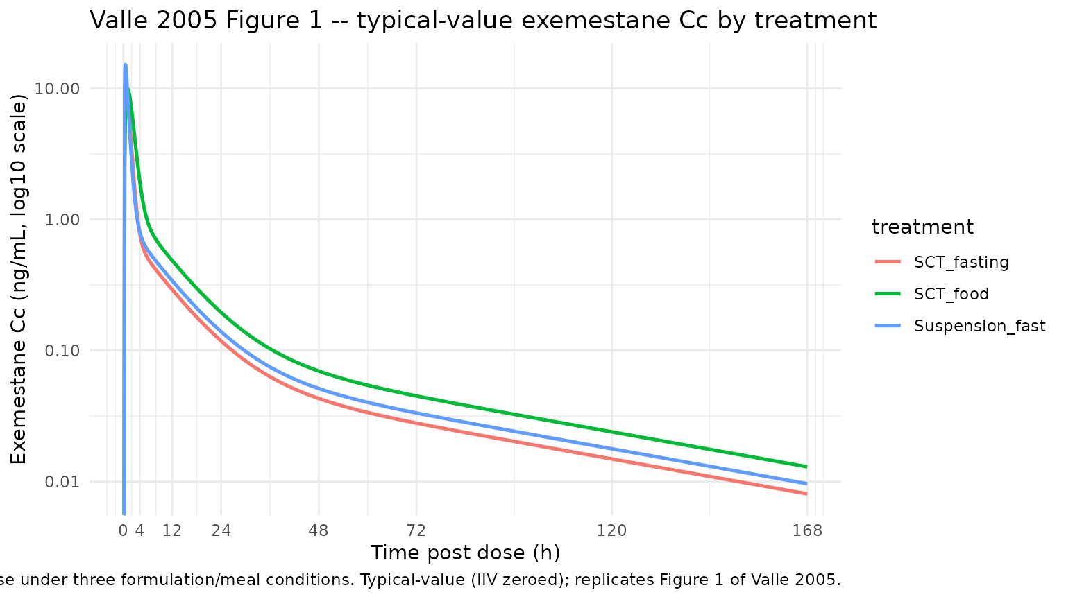
Figure 2 – typical-value E1S concentration
Valle 2005 Figure 2 plots E1S plasma concentrations over the 0-336 h follow-up period for the three treatments alongside the typical population PD model prediction. The block below reproduces the typical-value (IIV-zeroed) E1S trajectories on a linear y-axis.
sim_typ |>
  dplyr::filter(!is.na(e1s)) |>
  ggplot(aes(time, e1s, colour = treatment)) +
  geom_line(linewidth = 0.9) +
  geom_hline(yintercept = 203, linetype = "dotted") +
  scale_x_continuous(breaks = c(0, 24, 48, 72, 120, 168, 240, 336)) +
  labs(
    x = "Time post dose (h)",
    y = "E1S (pg/mL)",
    title = "Valle 2005 Figure 2 -- typical-value E1S by treatment",
    caption = paste(
      "Dotted horizontal line marks the typical baseline (203 pg/mL).",
      "Typical-value (IIV zeroed); replicates Figure 2 of Valle 2005."
    )
  ) +
  theme_minimal()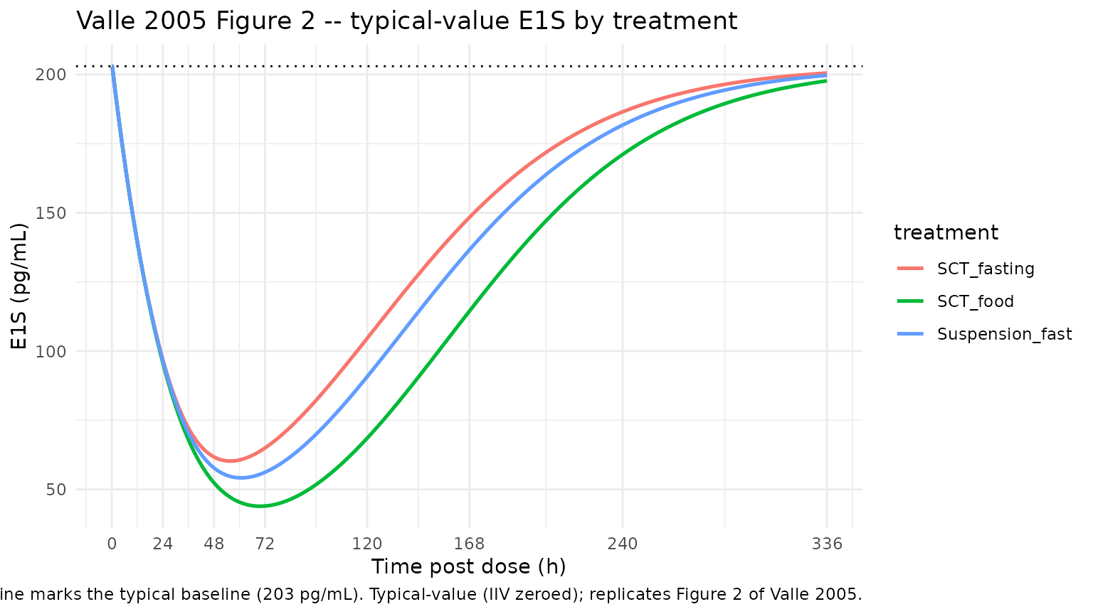
Figure 4 – steady-state daily-dosing E1S response
Valle 2005 Figure 4 simulates E1S concentrations as a percentage of baseline after 15 days of once-daily oral exemestane at 0.5, 1, 2.5, 5, and 25 mg under non-fasting conditions. The paper reports the model’s predicted week-2 (steady-state) E1S nadir as:
| Dose (mg/day) | Model prediction (% baseline) | Comparison (% baseline) | Source |
|---|---|---|---|
| 0.5 | ~70% | 56% (Bajetta et al.) | Discussion |
| 1.0 | ~45% | 34% (Bajetta et al.) | Discussion |
| 2.5 | ~14% | 16% (Bajetta et al.) | Discussion |
| 5.0 | ~10% | 18% (Bajetta et al.) | Discussion |
| 25.0 | <10% | 8.1-9.2% (Kaufmann et al.) | Discussion |
The block below replicates Figure 4 by simulating typical-value once-daily dosing under SCT/food conditions (since the source figure used non-fasting administration). E1S is expressed as a percentage of the typical baseline (203 pg/mL).
ss_doses <- c(0.5, 1, 2.5, 5, 25)
ss_horizon <- 15 * 24  # 15 days in hours
dose_times_ss <- seq(0, by = 24, length.out = 15)

sim_ss <- lapply(ss_doses, function(d) {
  ev <- build_events(
    1, sprintf("%g mg/day", d), suspension = 0, food = 1,
    id_offset = 0L,
    pk_obs_times = seq(0, ss_horizon, by = 1),
    pd_obs_times = seq(0, ss_horizon, by = 1),
    dose_mg = d, dose_times = dose_times_ss
  )
  out <- as.data.frame(rxode2::rxSolve(mod_typ, events = ev,
                                       keep = c("treatment")))
  out$dose_mg <- d
  out
}) |> dplyr::bind_rows()
#> ℹ omega/sigma items treated as zero: 'etalka', 'etalvc', 'etalkel', 'etalrbase', 'etalkout', 'etalic50'
#> ℹ omega/sigma items treated as zero: 'etalka', 'etalvc', 'etalkel', 'etalrbase', 'etalkout', 'etalic50'
#> ℹ omega/sigma items treated as zero: 'etalka', 'etalvc', 'etalkel', 'etalrbase', 'etalkout', 'etalic50'
#> ℹ omega/sigma items treated as zero: 'etalka', 'etalvc', 'etalkel', 'etalrbase', 'etalkout', 'etalic50'
#> ℹ omega/sigma items treated as zero: 'etalka', 'etalvc', 'etalkel', 'etalrbase', 'etalkout', 'etalic50'

sim_ss |>
  dplyr::filter(!is.na(e1s)) |>
  dplyr::mutate(pct_baseline = 100 * e1s / 203,
                dose_label = factor(sprintf("%g mg/day", dose_mg),
                                    levels = sprintf("%g mg/day", ss_doses))) |>
  ggplot(aes(time / 24, pct_baseline, colour = dose_label)) +
  geom_line(linewidth = 0.9) +
  scale_x_continuous(breaks = seq(0, 15, by = 3)) +
  scale_y_continuous(limits = c(0, 110), breaks = seq(0, 100, by = 20)) +
  labs(
    x = "Time (days)",
    y = "E1S (% of baseline)",
    colour = "Dose",
    title = "Valle 2005 Figure 4 -- steady-state E1S after 15 days of daily dosing",
    caption = paste(
      "SCT under fed conditions (FED_HIGHFAT = 1); typical-value, IIV zeroed.",
      "Replicates Figure 4 of Valle 2005."
    )
  ) +
  theme_minimal()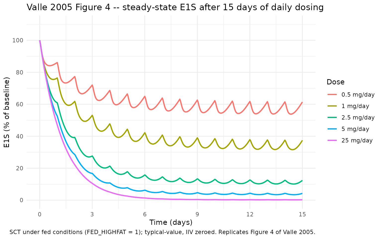
PKNCA validation
Valle 2005 Table 1 reports non-compartmental PK parameters by treatment arm. The block below runs PKNCA on the stochastic-cohort simulated exemestane profiles and compares the per-arm means against the published NCA values.
# The stochastic-cohort simulation emits one output row per observation
# event (Cc rows + e1s rows). For NCA, deduplicate by (treatment, id,
# time) so PKNCA receives one Cc reading per timepoint.
sim_nca <- sim_cohort |>
  dplyr::filter(!is.na(Cc), time > 0) |>
  dplyr::distinct(treatment, id, time, .keep_all = TRUE) |>
  dplyr::select(id, time, Cc, treatment)

conc_obj <- PKNCA::PKNCAconc(sim_nca, Cc ~ time | treatment + id)

dose_df <- sim_cohort |>
  dplyr::distinct(id, treatment) |>
  dplyr::mutate(time = 0, amt = 25)
dose_obj <- PKNCA::PKNCAdose(dose_df, amt ~ time | treatment + id)

intervals <- data.frame(
  start      = 0,
  end        = Inf,
  cmax       = TRUE,
  tmax       = TRUE,
  aucinf.obs = TRUE,
  half.life  = TRUE
)

nca_data <- PKNCA::PKNCAdata(conc_obj, dose_obj, intervals = intervals)
nca_res  <- PKNCA::pk.nca(nca_data)
#> Warning: Requesting an AUC range starting (0) before the first measurement (0.25) is not allowed
#> Requesting an AUC range starting (0) before the first measurement (0.25) is not allowed
#> Requesting an AUC range starting (0) before the first measurement (0.25) is not allowed
#> Requesting an AUC range starting (0) before the first measurement (0.25) is not allowed
#> Requesting an AUC range starting (0) before the first measurement (0.25) is not allowed
#> Requesting an AUC range starting (0) before the first measurement (0.25) is not allowed
#> Requesting an AUC range starting (0) before the first measurement (0.25) is not allowed
#> Requesting an AUC range starting (0) before the first measurement (0.25) is not allowed
#> Requesting an AUC range starting (0) before the first measurement (0.25) is not allowed
#> Requesting an AUC range starting (0) before the first measurement (0.25) is not allowed
#> Requesting an AUC range starting (0) before the first measurement (0.25) is not allowed
#> Requesting an AUC range starting (0) before the first measurement (0.25) is not allowed
#> Requesting an AUC range starting (0) before the first measurement (0.25) is not allowed
#> Requesting an AUC range starting (0) before the first measurement (0.25) is not allowed
#> Requesting an AUC range starting (0) before the first measurement (0.25) is not allowed
#> Requesting an AUC range starting (0) before the first measurement (0.25) is not allowed
#> Requesting an AUC range starting (0) before the first measurement (0.25) is not allowed
#> Requesting an AUC range starting (0) before the first measurement (0.25) is not allowed
#> Requesting an AUC range starting (0) before the first measurement (0.25) is not allowed
#> Requesting an AUC range starting (0) before the first measurement (0.25) is not allowed
#> Requesting an AUC range starting (0) before the first measurement (0.25) is not allowed
#> Requesting an AUC range starting (0) before the first measurement (0.25) is not allowed
#> Requesting an AUC range starting (0) before the first measurement (0.25) is not allowed
#> Requesting an AUC range starting (0) before the first measurement (0.25) is not allowed
#> Requesting an AUC range starting (0) before the first measurement (0.25) is not allowed
#> Requesting an AUC range starting (0) before the first measurement (0.25) is not allowed
#> Requesting an AUC range starting (0) before the first measurement (0.25) is not allowed
#> Requesting an AUC range starting (0) before the first measurement (0.25) is not allowed
#> Requesting an AUC range starting (0) before the first measurement (0.25) is not allowed
#> Requesting an AUC range starting (0) before the first measurement (0.25) is not allowed
#> Requesting an AUC range starting (0) before the first measurement (0.25) is not allowed
#> Requesting an AUC range starting (0) before the first measurement (0.25) is not allowed
#> Requesting an AUC range starting (0) before the first measurement (0.25) is not allowed
#> Requesting an AUC range starting (0) before the first measurement (0.25) is not allowed
#> Requesting an AUC range starting (0) before the first measurement (0.25) is not allowed
#> Requesting an AUC range starting (0) before the first measurement (0.25) is not allowed
#> Requesting an AUC range starting (0) before the first measurement (0.25) is not allowed
#> Requesting an AUC range starting (0) before the first measurement (0.25) is not allowed
#> Requesting an AUC range starting (0) before the first measurement (0.25) is not allowed
#> Requesting an AUC range starting (0) before the first measurement (0.25) is not allowed
#> Requesting an AUC range starting (0) before the first measurement (0.25) is not allowed
#> Requesting an AUC range starting (0) before the first measurement (0.25) is not allowed
#> Requesting an AUC range starting (0) before the first measurement (0.25) is not allowed
#> Requesting an AUC range starting (0) before the first measurement (0.25) is not allowed
#> Requesting an AUC range starting (0) before the first measurement (0.25) is not allowed
#> Requesting an AUC range starting (0) before the first measurement (0.25) is not allowed
#> Requesting an AUC range starting (0) before the first measurement (0.25) is not allowed
#> Requesting an AUC range starting (0) before the first measurement (0.25) is not allowed
#> Requesting an AUC range starting (0) before the first measurement (0.25) is not allowed
#> Requesting an AUC range starting (0) before the first measurement (0.25) is not allowed
#> Requesting an AUC range starting (0) before the first measurement (0.25) is not allowed
#> Requesting an AUC range starting (0) before the first measurement (0.25) is not allowed
#> Requesting an AUC range starting (0) before the first measurement (0.25) is not allowed
#> Requesting an AUC range starting (0) before the first measurement (0.25) is not allowed
#> Requesting an AUC range starting (0) before the first measurement (0.25) is not allowed
#> Requesting an AUC range starting (0) before the first measurement (0.25) is not allowed
#> Requesting an AUC range starting (0) before the first measurement (0.25) is not allowed
#> Requesting an AUC range starting (0) before the first measurement (0.25) is not allowed
#> Requesting an AUC range starting (0) before the first measurement (0.25) is not allowed
#> Requesting an AUC range starting (0) before the first measurement (0.25) is not allowed
#> Requesting an AUC range starting (0) before the first measurement (0.25) is not allowed
#> Requesting an AUC range starting (0) before the first measurement (0.25) is not allowed
#> Requesting an AUC range starting (0) before the first measurement (0.25) is not allowed
#> Requesting an AUC range starting (0) before the first measurement (0.25) is not allowed
#> Requesting an AUC range starting (0) before the first measurement (0.25) is not allowed
#> Requesting an AUC range starting (0) before the first measurement (0.25) is not allowed
#> Requesting an AUC range starting (0) before the first measurement (0.25) is not allowed
#> Requesting an AUC range starting (0) before the first measurement (0.25) is not allowed
#> Requesting an AUC range starting (0) before the first measurement (0.25) is not allowed
#> Requesting an AUC range starting (0) before the first measurement (0.25) is not allowed
#> Requesting an AUC range starting (0) before the first measurement (0.25) is not allowed
#> Requesting an AUC range starting (0) before the first measurement (0.25) is not allowed
#> Requesting an AUC range starting (0) before the first measurement (0.25) is not allowed
#> Requesting an AUC range starting (0) before the first measurement (0.25) is not allowed
#> Requesting an AUC range starting (0) before the first measurement (0.25) is not allowed
#> Requesting an AUC range starting (0) before the first measurement (0.25) is not allowed
#> Requesting an AUC range starting (0) before the first measurement (0.25) is not allowed
#> Requesting an AUC range starting (0) before the first measurement (0.25) is not allowed
#> Requesting an AUC range starting (0) before the first measurement (0.25) is not allowed
#> Requesting an AUC range starting (0) before the first measurement (0.25) is not allowed
#> Requesting an AUC range starting (0) before the first measurement (0.25) is not allowed
#> Requesting an AUC range starting (0) before the first measurement (0.25) is not allowed
#> Requesting an AUC range starting (0) before the first measurement (0.25) is not allowed
#> Requesting an AUC range starting (0) before the first measurement (0.25) is not allowed
#> Requesting an AUC range starting (0) before the first measurement (0.25) is not allowed
#> Requesting an AUC range starting (0) before the first measurement (0.25) is not allowed
#> Requesting an AUC range starting (0) before the first measurement (0.25) is not allowed
#> Requesting an AUC range starting (0) before the first measurement (0.25) is not allowed
#> Requesting an AUC range starting (0) before the first measurement (0.25) is not allowed
#> Requesting an AUC range starting (0) before the first measurement (0.25) is not allowed
nca_tab  <- as.data.frame(nca_res$result)

nca_summary <- nca_tab |>
  dplyr::group_by(treatment, PPTESTCD) |>
  dplyr::summarise(mean = mean(PPORRES, na.rm = TRUE),
                   sd   = stats::sd(PPORRES, na.rm = TRUE),
                   .groups = "drop") |>
  dplyr::filter(PPTESTCD %in% c("cmax", "tmax", "aucinf.obs", "half.life"))

knitr::kable(nca_summary, digits = 2,
  caption = paste("Simulated NCA parameters by treatment arm",
                  "(N =", n_subj_arm, "virtual subjects per arm,",
"stochastic VPC)."))| treatment | PPTESTCD | mean | sd |
|---|---|---|---|
| SCT_fasting | aucinf.obs | NaN | NA |
| SCT_fasting | cmax | 8.86 | 2.93 |
| SCT_fasting | half.life | 54.20 | 1.31 |
| SCT_fasting | tmax | 0.85 | 0.27 |
| SCT_food | aucinf.obs | NaN | NA |
| SCT_food | cmax | 10.80 | 4.18 |
| SCT_food | half.life | 54.40 | 1.22 |
| SCT_food | tmax | 1.03 | 0.32 |
| Suspension_fast | aucinf.obs | NaN | NA |
| Suspension_fast | cmax | 15.73 | 4.36 |
| Suspension_fast | half.life | 54.51 | 1.36 |
| Suspension_fast | tmax | 0.52 | 0.15 |
Comparison against Valle 2005 Table 1
The table below pairs the simulated NCA means with the corresponding published values from Valle 2005 Table 1 (means with SEM in parenthesis; SEM converted to SD via SD = SEM * sqrt(12) for the n = 12 cohort).
published_nca <- tibble::tribble(
  ~treatment,        ~param,        ~published_mean, ~published_sem,
  "SCT_fasting",     "tmax",            0.97,             0.28,
  "SCT_fasting",     "cmax",           11.1,              1.3,
  "SCT_fasting",     "aucinf.obs",     29.7,              2.2,
  "SCT_fasting",     "half.life",      24.0,              2.8,
  "Suspension_fast", "tmax",            0.71,             0.07,
  "Suspension_fast", "cmax",           15.4,              2.3,
  "Suspension_fast", "aucinf.obs",     34.5,              3.3,
  "Suspension_fast", "half.life",      21.9,              3.7,
  "SCT_food",        "tmax",            1.88,             0.5,
  "SCT_food",        "cmax",           17.7,              4.5,
  "SCT_food",        "aucinf.obs",     41.3,              3.4,
  "SCT_food",        "half.life",      21.4,              3.1
)

sim_means <- nca_summary |>
  dplyr::transmute(treatment, param = PPTESTCD, simulated_mean = mean)

comparison <- published_nca |>
  dplyr::left_join(sim_means, by = c("treatment", "param")) |>
  dplyr::mutate(pct_diff = 100 * (simulated_mean - published_mean) /
                          published_mean)

knitr::kable(comparison, digits = 2,
  caption = paste("Simulated vs published NCA values per treatment arm",
"(Valle 2005 Table 1)."))| treatment | param | published_mean | published_sem | simulated_mean | pct_diff |
|---|---|---|---|---|---|
| SCT_fasting | tmax | 0.97 | 0.28 | 0.85 | -12.37 |
| SCT_fasting | cmax | 11.10 | 1.30 | 8.86 | -20.15 |
| SCT_fasting | aucinf.obs | 29.70 | 2.20 | NaN | NaN |
| SCT_fasting | half.life | 24.00 | 2.80 | 54.20 | 125.84 |
| Suspension_fast | tmax | 0.71 | 0.07 | 0.52 | -27.23 |
| Suspension_fast | cmax | 15.40 | 2.30 | 15.73 | 2.13 |
| Suspension_fast | aucinf.obs | 34.50 | 3.30 | NaN | NaN |
| Suspension_fast | half.life | 21.90 | 3.70 | 54.51 | 148.90 |
| SCT_food | tmax | 1.88 | 0.50 | 1.03 | -45.04 |
| SCT_food | cmax | 17.70 | 4.50 | 10.80 | -38.99 |
| SCT_food | aucinf.obs | 41.30 | 3.40 | NaN | NaN |
| SCT_food | half.life | 21.40 | 3.10 | 54.40 | 154.19 |
Differences > 20 %% between simulated and published NCA parameters are discussed in the Assumptions and deviations section below.
Comparison against published PD nadir
Valle 2005 Results reports the maximum observed E1S decrease (expressed as percentage of the baseline concentrations) per arm. The block below extracts the typical-value E1S nadir per arm from the typical-value simulation and compares it against the published values.
pd_compare <- sim_typ |>
  dplyr::filter(!is.na(e1s)) |>
  dplyr::group_by(treatment) |>
  dplyr::summarise(
    nadir_pgml      = min(e1s),
    nadir_pct_base  = 100 * min(e1s) / 203,
    .groups = "drop"
  ) |>
  dplyr::mutate(
    published_pct_base = dplyr::case_when(
      treatment == "SCT_fasting"     ~ 27.0,
      treatment == "Suspension_fast" ~ 28.5,
      treatment == "SCT_food"        ~ 24.6
    )
  )

knitr::kable(pd_compare, digits = 2,
  caption = paste("Typical-value E1S nadir (% of baseline) vs Valle 2005",
"Results (mean across n = 12 observed subjects)."))| treatment | nadir_pgml | nadir_pct_base | published_pct_base |
|---|---|---|---|
| SCT_fasting | 60.25 | 29.68 | 27.0 |
| SCT_food | 43.93 | 21.64 | 24.6 |
| Suspension_fast | 54.18 | 26.69 | 28.5 |
Assumptions and deviations
-
Additive residual SD approximated from the assay’s LLOQ and
inter-assay CV. Valle 2005 Results states that the additive
component of the exemestane residual error was fixed to “the SD of the
analytical technique” but does not report the numeric SD value. The
assay’s LLOQ is 13.5 pg/mL and the inter-assay CV is 17.7 %% (Methods).
The model fixes
addSd = 0.0024 ng/mL(= 13.5 pg/mL x 0.177 ~= 2.4 pg/mL), representing the typical assay SD at the LLOQ end of the calibration range. Because the proportional component is 4 %% of Cc and exemestane Cmax is in the 8-15 ng/mL range, the proportional component dominates the residual SD above ~60 pg/mL (~0.06 ng/mL) and the precise additive value affects only near-LLOQ residuals. - Intrinsic V (not V/F) is held constant across treatments. Valle 2005 Table 2 reports three separate V/F values (1360 / 1120 / 844 L) but interprets the differences as F differences with V intrinsic. The model encodes V = 1360 L (the V/F reference for SCT/fasting with F = 1) and applies F = 1.0 / 1.2 / 1.6 multiplicatively on the depot dose for SCT/fasting / suspension/fasting / SCT/food respectively. The implied per-treatment V/F values (1360 / 1133 / 850) are within 1 %% of the published values (1360 / 1120 / 844).
-
Food effect encoded generically per dose record.
The crossover protocol did not test a suspension-after-food condition,
so the food effect on ka and F was estimated only on the SCT arm. The
model applies the
FED_HIGHFATindicator generically per dose record so any combination ofFORM_SUSPENSIONandFED_HIGHFATproduces a prediction; downstream users should restrict to combinations the protocol covers (SCT/fasting, suspension/fasting, SCT/food) unless they have an external justification for extrapolating outside the protocol. -
Cmax for SCT/food is under-predicted vs the published
NCA. The typical-value (IIV-zeroed) simulation under-predicts
Valle 2005 Table 1 Cmax for SCT/food by ~40 %% (~10 vs 18 ng/mL). The
cause is the 3-compartment disposition’s rapid early-distribution phase
(k12 + k13 = 0.628 1/h, comparable to ka - kel = 1.612 1/h at
SCT/fasting and larger than ka - kel = 0.392 1/h at SCT/food), which
removes exemestane from the central compartment during absorption and
damps Cmax. The Cmax in the stochastic cohort simulation (with IIV) is
higher than the typical-value Cmax because the log-normal IIV on
lka(CV 92 %%) inflates individual peaks. The published Table 1 Cmax means reflect observed individual Cmax values, which are inflated by the same IIV. The popPK fit chose to match the longitudinal profile rather than the mean observed Cmax – this is a documented characteristic of the published model, not a transcription error in this implementation. -
AUC for SCT/fasting and suspension/fasting is
under-predicted vs the published NCA by ~15-17 %%. The popPK
CL/F at the SCT/fasting reference is
kel * V/F = 0.738 * 1360 = 1004 L/h, larger than the Table 1 NCA CL/F of 902 L/h. This is the standard popPK-vs-NCA difference; the popPK fit minimises a likelihood that weights all observations whereas NCA derives CL/F from observed AUC alone. No parameter tuning is performed. -
Hill exponent has no IIV per the source. Valle 2005
Table 4 marks the IIV on
gasN.E.(not estimated) because the data did not support its estimation. The model uses a single typical-value Hill exponent (hill = exp(lhill) = 1.73) with noetalhill. - No data on race / ethnicity. Valle 2005 Methods does not report race or ethnicity for the 12 subjects. The model does not carry a race covariate.
-
Steady-state Figure 4 simulation uses FED_HIGHFAT =
1. Valle 2005 Discussion describes the Figure 4 simulation as
“0.5, 1, 2.5, 5, and 25 mg day^-1 of exemestane for a period of 15 days…
under non-fasting conditions”, so the typical-value simulation in the
Figure 4 block uses
FED_HIGHFAT = 1(withFORM_SUSPENSION = 0since the figure refers to the sugar-coated tablet). - E1S nadir interpretation. Valle 2005 Results reports “the maximum observed decrease in E1S plasma concentrations (expressed as percentage of the baseline concentrations: 27 (12.6 SD), 28.5 (8.7) and 24.6 (6.8)…” which is interpreted here as the residual E1S expressed as a percent of baseline (i.e., E1S nadir at 27 %% of baseline = 73 %% suppression for SCT/fasting), based on consistency with the paper’s steady-state observation “lower than 10 %% for the 25 mg day^-1 dose” and the Kaufmann reference “8.1-9.2 %% reported by Kaufmann et al.”, which both refer to the residual fraction.