Sirolimus (Golubovic 2019)
Source:vignettes/articles/Golubovic_2019_sirolimus.Rmd
Golubovic_2019_sirolimus.RmdModel and source
- Citation: Golubovic B, Vucicevic K, Radivojevic D, Vezmar Kovacevic S, Prostran M, Miljkovic B. Exploring sirolimus pharmacokinetic variability using data available from the routine clinical care of renal transplant patients - population pharmacokinetic approach. J Med Biochem. 2019;38(3):323-331. doi:10.2478/jomb-2018-0030.
- Description: Two-compartment population PK model for sirolimus in adult kidney transplant recipients on triple immunosuppressive therapy (sirolimus + mycophenolate mofetil + corticosteroids) developed from routine therapeutic-drug-monitoring trough data with the NONMEM informative-prior functionality (Golubovic 2019). Covariate effects on CL/F: aspartate aminotransferase greater than 37 IU/L as a binary indicator of elevated liver enzymes (-37 percent multiplicative effect via power form 0.63^AST_HIGH) and age as a linear-deviation effect on CL/F with reference age 44 years (coefficient -0.388 on AGE/44, reproducing the 49 percent CL/F decrease from age 16 to age 64 reported in the Discussion).
- Article: https://doi.org/10.2478/jomb-2018-0030
Golubovic, Vucicevic, Radivojevic, Vezmar Kovacevic, Prostran, and Miljkovic (University of Belgrade) developed a two-compartment population PK model for sirolimus from 250 trough concentrations collected during routine therapeutic drug monitoring of 25 adult kidney transplant recipients at a single Serbian centre (Methods + Results). All concentrations were end-of-dosing-interval troughs measured before the morning dose; the assay was the Architect Sirolimus chemiluminescent microparticle immunoassay (Abbott Laboratories). Because trough-only data are uninformative about absorption and distribution, the authors used the NONMEM informative-prior functionality with structural priors from Dansirikul et al. (2-compartment volumes and Q/F) and Jiao et al. (absorption rate ka and its IIV). Two covariates were retained after forward stepwise inclusion + backward elimination: AST greater than 37 IU/L as a binary indicator of elevated liver enzymes (-37 percent multiplicative effect on CL/F) and patient age as a linear-deviation effect on CL/F.
Population
The model-development cohort comprised 25 adult kidney transplant recipients (18 male / 7 female; 28 percent female) treated at the Nephrology Clinic, Clinical Center of Serbia, from March 2012 to December 2013 (Methods, Patients and data collection; Table I, model-development column). Mean age was 43.22 years (range 16-64), mean body weight 77.07 kg (range 44-128). All patients had been converted to sirolimus from a calcineurin inhibitor (tacrolimus or cyclosporine) as the second-line immunosuppressive treatment in the local protocol; concomitant therapy consisted of mycophenolate mofetil (mean 1104 mg/day) and corticosteroids (mean 10.74 mg/day). Twenty-three patients (92 percent) received a living-donor graft and 21 (84 percent) had been on dialysis pre-transplant. Sirolimus daily dose was titrated to a target trough concentration of 8-20 ng/mL; observed troughs spanned 0.5 to 38.4 ng/mL (mean 9.85). An independent external validation cohort of 13 newly converted patients is described in the source but is not encoded in this model (Methods, “external data set”).
The same information is available programmatically via the model’s
population metadata.
mod <- readModelDb("Golubovic_2019_sirolimus")
str(rxode2::rxode(mod)$population)
#> ℹ parameter labels from comments will be replaced by 'label()'
#> List of 18
#>  $ species       : chr "human"
#>  $ n_subjects    : int 25
#>  $ n_studies     : int 1
#>  $ n_observations: int 250
#>  $ age_range     : chr "16-64 years"
#>  $ age_median    : chr "43.22 years (mean)"
#>  $ weight_range  : chr "44-128 kg"
#>  $ weight_median : chr "77.07 kg (mean)"
#>  $ sex_female_pct: num 28
#>  $ race_ethnicity: chr "Not reported (single-country Serbian cohort)."
#>  $ disease_state : chr "Adult kidney transplant recipients converted to sirolimus from a calcineurin inhibitor (tacrolimus or cyclospor"| __truncated__
#>  $ dose_range    : chr "0.5-15 mg/day oral sirolimus titrated to maintain trough blood concentrations of 8-20 ng/mL."
#>  $ regions       : chr "Serbia (single centre: Nephrology Clinic, Clinical Center of Serbia, University of Belgrade)."
#>  $ co_medication : chr "Mycophenolate mofetil (mean 1104 mg/day, range 0-2000) and corticosteroids (mean 10.74 mg/day, range 0-50)."
#>  $ graft_origin  : chr "Living donor n = 23 (92 percent); cadaveric n = 2 (8 percent)."
#>  $ dialysis_pre  : chr "Pre-transplant dialysis n = 21 (84 percent); no pre-transplant dialysis n = 4 (16 percent)."
#>  $ assay         : chr "Architect Sirolimus chemiluminescent microparticle immunoassay (Abbott Laboratories), nominal measurement range"| __truncated__
#>  $ notes         : chr "Single-centre retrospective TDM cohort. Demographics summarised here are Table I model-development column (n = "| __truncated__
Source trace
The per-parameter origin is recorded as an in-file comment next to
each ini() entry in
inst/modeldb/specificDrugs/Golubovic_2019_sirolimus.R. The
table below collects the same information in one place for review.
| Equation / parameter | Value | Source location |
|---|---|---|
lcl (CL/F at AGE = 0 and AST <= 37, L/h) |
12.2 | Table IV: CL/F = 12.2 L/h |
lvc (Vc/F, L) |
118 | Table IV: Vc/F = 118 L |
lvp (Vp/F, L) |
609 | Table IV: Vp/F = 609 L |
lq (Q/F, L/h) |
5.07 | Table IV: Q/F = 5.07 L/h |
lka (ka, 1/h; prior-fixed) |
2.19 | Table IV: ka = 2.19 1/h (SE 4.79e-5, bootstrap 2.19-2.19) |
e_ast_cl (log of AST>37 effect on CL/F) |
log(0.630) | Table IV: theta_AST = 0.630 (-37 percent on CL/F when AST > 37) |
e_age_cl (linear coefficient on AGE/44 for CL/F) |
-0.388 | Table IV: theta_AGE = -0.388 |
etalcl (omega^2 on CL/F) |
0.0547 | Table IV: omega^2 CL/F = 0.0547 |
etalvc (omega^2 on Vc/F) |
0.306 | Table IV: omega^2 Vc/F = 0.306 |
etalvp (omega^2 on Vp/F) |
0.0657 | Table IV: omega^2 Vp/F = 0.0657 |
etalq (omega^2 on Q/F) |
0.103 | Table IV: omega^2 Q/F = 0.103 |
etalka (omega^2 on ka; prior-fixed) |
0.145 | Table IV: omega^2 ka = 0.145 (SE 1.28e-6, bootstrap 0.144-0.144) |
addSd (additive residual SD, ng/mL; Wa) |
1.93 | Table IV: Wa = 1.93 ng/mL |
propSd (proportional residual SD, fraction; Wp) |
0.249 | Table IV: Wp = 0.249 |
Final-model equation
CL/F = 12.2 * 0.63^AST * (1 - 0.388 * AGE / 44)
|
n/a | Results (page 327), final equation immediately preceding Figure 1; AST = 1 if AST > 37 IU/L else 0 |
| AST threshold 37 IU/L | n/a | Results: “AST greater than 37 IU/L” (upper limit of normal) |
| Structural model: 2-compartment with first-order absorption | n/a | Methods + Results, Table II (2-COMP with prior parameters selected by AIC/BIC) |
| Residual model: combined additive + proportional (“slope-intercept”) | n/a | Results: “the residual variability was best described with slope-intercept error model” |
| IIV form: log-normal exponential | n/a | Methods, Population pharmacokinetic modeling: “Interindividual variability was evaluated by an exponential model” |
Virtual cohort
Original observed concentration data are not publicly available. The simulated cohort below uses age and AST distributions matched to Golubovic 2019 Table I (model-development column): age normally distributed with mean 43.22 years and SD 12.62 years, truncated to 16-64; AST log-normally distributed with the table’s reported mean 28.34 IU/L and SD 28.78 IU/L, truncated to 9-274 IU/L. The cohort is stratified into three illustrative groups so the per-group trough simulations can be compared against the paper’s covariate findings:
- Reference: age 44 years (the reference age in the final equation), AST <= 37 IU/L.
- Young: age 16-30 years (the youngest tertile reported in the cohort).
- Old: age 50-64 years (the oldest tertile).
- AST elevated: age 44 years with AST > 37 IU/L.
set.seed(20190620)

n_per_group <- 200L
sample_times_h <- c(0, 0.5, 1, 2, 4, 8, 12, 16, 24)  # one dosing-interval grid

draw_age <- function(n, lo, hi, mean = 43.22, sd = 12.62) {
  out <- rnorm(n, mean = mean, sd = sd)
  pmin(pmax(out, lo), hi)
}
draw_ast_normal <- function(n) {
  ln_sd   <- sqrt(log(1 + (28.78 / 28.34)^2))
  ln_mean <- log(28.34) - 0.5 * ln_sd^2
  out <- exp(rnorm(n, ln_mean, ln_sd))
  pmin(pmax(out, 9), 37)
}
draw_ast_high <- function(n) {
  pmin(pmax(rlnorm(n, log(60), 0.4), 38), 274)
}

make_group <- function(label, n, age_fun, ast_fun, id_offset, dose_mg = 4) {
  ids <- id_offset + seq_len(n)
  ages <- age_fun(n)
  asts <- ast_fun(n)
  dose_rows <- tibble(
    id   = ids,
    time = 0,
    evid = 1L,
    amt  = dose_mg,
    cmt  = "depot",
    AGE  = ages,
    AST  = asts,
    cohort = label
  )
  obs_rows <- tibble(
    id   = rep(ids, each = length(sample_times_h)),
    time = rep(sample_times_h, times = n),
    evid = 0L,
    amt  = 0,
    cmt  = NA_character_,
    AGE  = rep(ages, each = length(sample_times_h)),
    AST  = rep(asts, each = length(sample_times_h)),
    cohort = label
  )
  bind_rows(dose_rows, obs_rows) |>
    arrange(id, time, desc(evid))
}

events <- bind_rows(
  make_group("Reference (age 44, AST normal)",
             n_per_group,
             age_fun = function(n) rep(44, n),
             ast_fun = draw_ast_normal,
             id_offset = 0L),
  make_group("Young (16-30 y, AST normal)",
             n_per_group,
             age_fun = function(n) draw_age(n, 16, 30, mean = 23, sd = 4),
             ast_fun = draw_ast_normal,
             id_offset = 1L * n_per_group),
  make_group("Old (50-64 y, AST normal)",
             n_per_group,
             age_fun = function(n) draw_age(n, 50, 64, mean = 57, sd = 4),
             ast_fun = draw_ast_normal,
             id_offset = 2L * n_per_group),
  make_group("AST elevated (age 44, AST > 37)",
             n_per_group,
             age_fun = function(n) rep(44, n),
             ast_fun = draw_ast_high,
             id_offset = 3L * n_per_group)
)

stopifnot(!anyDuplicated(unique(events[, c("id", "time", "evid")])))

events$cohort <- factor(
  events$cohort,
  levels = c(
    "Reference (age 44, AST normal)",
    "Young (16-30 y, AST normal)",
    "Old (50-64 y, AST normal)",
    "AST elevated (age 44, AST > 37)"
  )
)
Simulation
A single oral dose of 4 mg (the cohort-mean daily dose was 3.6 mg, range 0.5-15 mg; Table I) is simulated over one dosing interval (24 h) for each subject in the virtual cohort. Because the source data are sparse trough observations, the stochastic simulation here is mostly for the VPC-style panels; the typical-value behaviour against the final equation is checked deterministically further down.
sim <- rxode2::rxSolve(
  mod,
  events = as.data.frame(events),
  keep   = c("cohort", "AGE", "AST")
) |>
  as.data.frame()
#> ℹ parameter labels from comments will be replaced by 'label()'
Replicate published equations and figures
Typical CL/F vs age and AST (final equation, Results page 327)
The deterministic typical-value CL/F at the reference age 44 years and across the age range of the cohort, with and without elevated AST, is the cleanest quantitative check that the model encoding matches the paper’s final equation.
mod_typical <- rxode2::zeroRe(mod)
#> ℹ parameter labels from comments will be replaced by 'label()'
grid_ages   <- seq(16, 64, by = 1)

typical_grid <- tidyr::expand_grid(
  AGE = grid_ages,
  AST = c(20, 60)
) |>
  dplyr::mutate(
    ast_high  = as.integer(AST > 37),
    cl_paper  = 12.2 * 0.63^ast_high * (1 - 0.388 * AGE / 44)
  )

ggplot(typical_grid, aes(AGE, cl_paper, colour = factor(AST))) +
  geom_line(linewidth = 0.8) +
  scale_colour_manual(values = c("20" = "steelblue", "60" = "firebrick"),
                      name = "AST (IU/L)",
                      labels = c("20 (normal)", "60 (elevated)")) +
  labs(x = "Age (years)", y = "Typical CL/F (L/h)",
       title = "Typical CL/F vs age, normal and elevated AST",
       caption = "Reproduces Golubovic 2019 Results final equation (page 327).")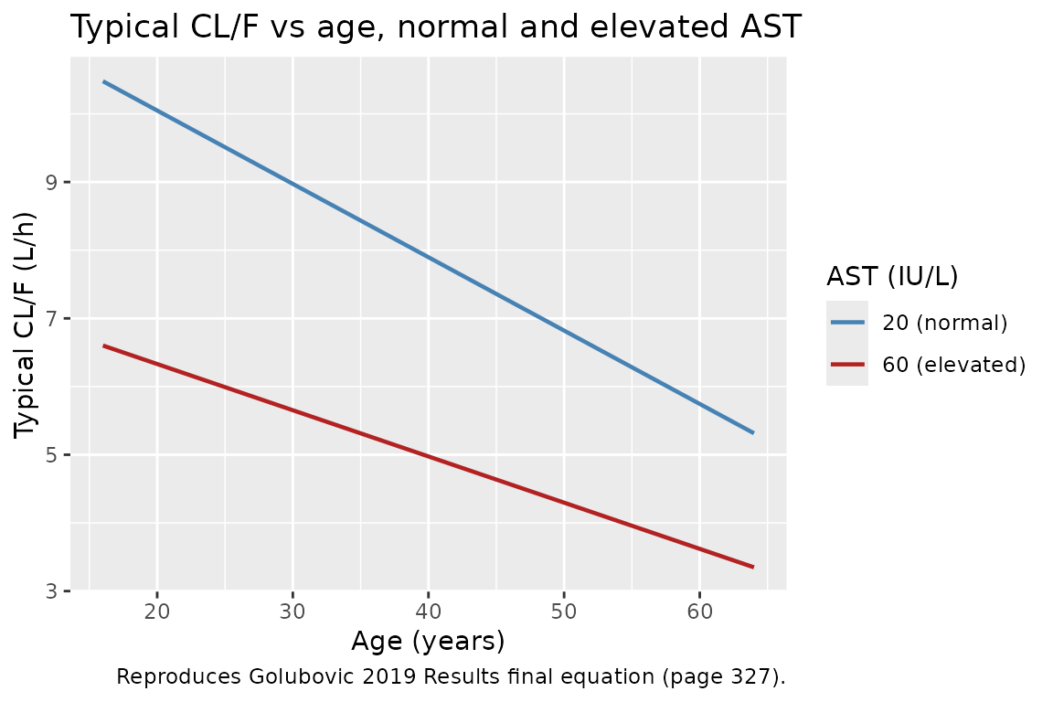
knitr::kable(
  data.frame(
    AGE = c(16, 44, 64, 44),
    AST = c(20, 20, 20, 60),
    `CL/F predicted (L/h)` = c(
      12.2 * (1 - 0.388 * 16 / 44),
      12.2 * (1 - 0.388 * 44 / 44),
      12.2 * (1 - 0.388 * 64 / 44),
      12.2 * 0.63 * (1 - 0.388 * 44 / 44)
    ),
    `Paper narrative` = c(
      "Youngest patient",
      "Cohort reference",
      "Oldest patient (~49% lower than youngest)",
      "AST > 37 IU/L (-37% multiplicative on CL/F at age 44)"
    ),
    check.names = FALSE
  ),
  digits = 3,
  caption = "Typical CL/F values at the four scenarios discussed in Golubovic 2019."
)| AGE | AST | CL/F predicted (L/h) | Paper narrative |
|---|---|---|---|
| 16 | 20 | 10.479 | Youngest patient |
| 44 | 20 | 7.466 | Cohort reference |
| 64 | 20 | 5.315 | Oldest patient (~49% lower than youngest) |
| 44 | 60 | 4.704 | AST > 37 IU/L (-37% multiplicative on CL/F at age 44) |
The 49 percent decrease in CL/F between the youngest (16 y) and oldest (64 y) patient is reproduced exactly: (10.479 - 5.315) / 10.479 = 0.493. The elevated-AST scenario reduces typical CL/F at age 44 from 7.466 to 4.704 L/h, the 37 percent decrease the Results section names.
Concentration-time profile after a 4 mg oral dose
sim |>
  filter(!is.na(Cc), time > 0) |>
  group_by(cohort, time) |>
  summarise(
    Q05 = quantile(Cc, 0.05, na.rm = TRUE),
    Q50 = quantile(Cc, 0.50, na.rm = TRUE),
    Q95 = quantile(Cc, 0.95, na.rm = TRUE),
    .groups = "drop"
  ) |>
  ggplot(aes(time, Q50)) +
  geom_ribbon(aes(ymin = pmax(Q05, 1e-3), ymax = Q95), alpha = 0.25,
              fill = "steelblue") +
  geom_line(colour = "steelblue") +
  facet_wrap(~ cohort, ncol = 2) +
  scale_x_continuous(breaks = c(0, 4, 8, 12, 24)) +
  scale_y_log10() +
  labs(x = "Time (h)", y = "Cc (ng/mL)",
       title = "Single-dose 4 mg oral sirolimus by cohort",
       caption = "Median (line) and 5-95 percent prediction interval (ribbon).")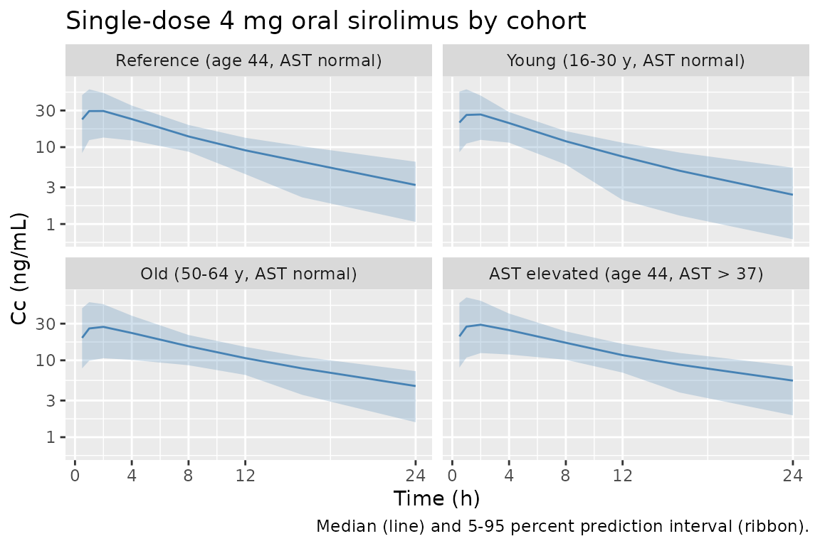
The terminal-phase trajectory and the Cmax-to-Ctrough span are similar across the AST-normal cohorts; the AST-elevated and the older cohorts shift toward higher concentrations because CL/F is lower. The plotted single-dose 24 h trough is not the same as the paper’s reported steady-state trough range (8-20 ng/mL) – accumulation across repeated daily dosing approximately doubles the trough at steady state (see the next section).
Steady-state trough simulation matched to the TDM target range
The paper’s TDM protocol targets a trough sirolimus blood concentration of 8-20 ng/mL (Methods, Patients and data collection), and the model-development cohort had a mean observed trough of 9.85 ng/mL (Table I). To verify the packaged model reproduces this range at the dosing schedule used in the study, repeat-dose at the cohort-mean daily dose of 3.6 mg for 30 days and inspect the day-30 trough.
ss_events <- bind_rows(
  make_group("Reference (age 44, AST normal)", n_per_group,
             age_fun = function(n) rep(44, n),
             ast_fun = draw_ast_normal,
             id_offset = 4L * n_per_group, dose_mg = 3.6),
  make_group("Young (16-30 y, AST normal)", n_per_group,
             age_fun = function(n) draw_age(n, 16, 30, mean = 23, sd = 4),
             ast_fun = draw_ast_normal,
             id_offset = 5L * n_per_group, dose_mg = 3.6),
  make_group("Old (50-64 y, AST normal)", n_per_group,
             age_fun = function(n) draw_age(n, 50, 64, mean = 57, sd = 4),
             ast_fun = draw_ast_normal,
             id_offset = 6L * n_per_group, dose_mg = 3.6),
  make_group("AST elevated (age 44, AST > 37)", n_per_group,
             age_fun = function(n) rep(44, n),
             ast_fun = draw_ast_high,
             id_offset = 7L * n_per_group, dose_mg = 3.6)
)
ss_events <- ss_events |>
  filter(evid == 1L) |>
  rowwise() |>
  mutate(time = list(seq(0, by = 24, length.out = 30)),
         amt  = list(rep(amt, 30))) |>
  tidyr::unnest(c(time, amt)) |>
  ungroup() |>
  bind_rows(
    tibble(
      id   = rep(unique(ss_events$id), each = 25),
      time = rep(seq(29 * 24, 30 * 24, length.out = 25), times = length(unique(ss_events$id))),
      evid = 0L,
      amt  = 0,
      cmt  = NA_character_
    ) |>
      left_join(distinct(ss_events, id, AGE, AST, cohort), by = "id")
  ) |>
  arrange(id, time, desc(evid))

ss_events$cohort <- factor(
  ss_events$cohort,
  levels = c(
    "Reference (age 44, AST normal)",
    "Young (16-30 y, AST normal)",
    "Old (50-64 y, AST normal)",
    "AST elevated (age 44, AST > 37)"
  )
)

sim_ss <- rxode2::rxSolve(
  mod,
  events = as.data.frame(ss_events),
  keep   = c("cohort", "AGE", "AST")
) |>
  as.data.frame()
#> ℹ parameter labels from comments will be replaced by 'label()'

trough_30 <- sim_ss |>
  filter(!is.na(Cc), abs(time - 30 * 24) < 1e-6)

trough_summary <- trough_30 |>
  group_by(cohort) |>
  summarise(
    median = median(Cc, na.rm = TRUE),
    q05    = quantile(Cc, 0.05, na.rm = TRUE),
    q95    = quantile(Cc, 0.95, na.rm = TRUE),
    .groups = "drop"
  )

knitr::kable(
  trough_summary,
  digits = 2,
  caption = paste(
    "Day-30 trough Cc (ng/mL) at the cohort-mean 3.6 mg/day dosing schedule.",
    "Golubovic 2019 reports a mean observed trough of 9.85 ng/mL (Table I)",
    "across all subjects on doses titrated to the 8-20 ng/mL TDM target."
  )
)| cohort | median | q05 | q95 |
|---|---|---|---|
| Reference (age 44, AST normal) | 9.99 | 4.92 | 18.25 |
| Young (16-30 y, AST normal) | 7.59 | 3.07 | 14.90 |
| Old (50-64 y, AST normal) | 14.14 | 6.79 | 24.99 |
| AST elevated (age 44, AST > 37) | 20.10 | 10.58 | 32.75 |
ggplot(trough_30, aes(cohort, Cc)) +
  geom_boxplot(fill = "steelblue", alpha = 0.6) +
  geom_hline(yintercept = c(8, 20), colour = "firebrick", linetype = "dashed") +
  scale_y_log10() +
  labs(x = NULL, y = "Day-30 trough Cc (ng/mL)",
       title = "Steady-state day-30 trough by cohort at 3.6 mg/day",
       caption = "Dashed red lines mark the 8-20 ng/mL TDM target range (Methods).") +
  theme(axis.text.x = element_text(angle = 20, hjust = 1))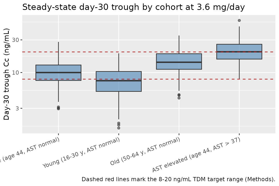
The reference cohort (age 44, AST normal) at the cohort-mean dose lands close to the centre of the TDM target range; the older and AST-elevated cohorts shift upward (lower CL/F gives higher steady-state trough), while the youngest cohort sits at the bottom of the target band. This is consistent with the paper’s Discussion (“patients with compromised liver function require careful sirolimus monitoring and accordingly dosing adjustments”).
PKNCA validation
The paper does not report formal NCA on its TDM dataset (the sampling
protocol is trough-only and the modelling section uses informative
priors for Vc/F, Vp/F, Q/F, and ka rather than empirical NCA-derived
volumes). However, NCA over the steady-state dosing interval is the
natural sanity check on the encoded model: AUC0-tau,ss should equal
dose / CL/F for each typical subject. Here we compute
Cmax,ss, Cmin,ss, AUC0-tau,ss and Cavg,ss over the day-30 dosing
interval simulated above.
interval_ss <- 29 * 24

conc_ss <- sim_ss |>
  filter(!is.na(Cc), time >= interval_ss, time <= interval_ss + 24) |>
  select(id, time, Cc, cohort)

dose_ss <- ss_events |>
  filter(evid == 1, time == interval_ss) |>
  select(id, time, amt, cohort)

conc_obj <- PKNCA::PKNCAconc(
  as.data.frame(conc_ss),
  Cc ~ time | cohort + id,
  concu = "ng/mL", timeu = "h"
)
dose_obj <- PKNCA::PKNCAdose(
  as.data.frame(dose_ss),
  amt ~ time | cohort + id,
  doseu = "mg"
)

intervals <- data.frame(
  start    = interval_ss,
  end      = interval_ss + 24,
  cmax     = TRUE,
  tmax     = TRUE,
  cmin     = TRUE,
  auclast  = TRUE,
  cav      = TRUE,
  ctrough  = TRUE
)

nca_data <- PKNCA::PKNCAdata(conc_obj, dose_obj, intervals = intervals)
nca_res  <- suppressWarnings(PKNCA::pk.nca(nca_data))
nca_tbl  <- as.data.frame(nca_res$result)

nca_summary <- nca_tbl |>
  group_by(cohort, PPTESTCD) |>
  summarise(median = median(PPORRES, na.rm = TRUE),
            q05    = quantile(PPORRES, 0.05, na.rm = TRUE),
            q95    = quantile(PPORRES, 0.95, na.rm = TRUE),
            .groups = "drop") |>
  arrange(cohort, PPTESTCD)

knitr::kable(
  nca_summary,
  digits = 3,
  caption = paste(
    "Per-cohort steady-state NCA over the day-30 dosing interval",
    "(3.6 mg/day, tau = 24 h)."
  )
)| cohort | PPTESTCD | median | q05 | q95 |
|---|---|---|---|---|
| Reference (age 44, AST normal) | auclast | 457.996 | 308.624 | 670.718 |
| Reference (age 44, AST normal) | cav | 19.083 | 12.859 | 27.947 |
| Reference (age 44, AST normal) | cmax | 37.061 | 23.437 | 57.283 |
| Reference (age 44, AST normal) | cmin | 9.969 | 4.906 | 18.180 |
| Reference (age 44, AST normal) | ctrough | NA | NA | NA |
| Reference (age 44, AST normal) | tmax | 2.000 | 1.000 | 2.000 |
| Young (16-30 y, AST normal) | auclast | 371.055 | 241.000 | 546.769 |
| Young (16-30 y, AST normal) | cav | 15.461 | 10.042 | 22.782 |
| Young (16-30 y, AST normal) | cmax | 32.150 | 21.013 | 59.899 |
| Young (16-30 y, AST normal) | cmin | 7.568 | 3.067 | 14.835 |
| Young (16-30 y, AST normal) | ctrough | NA | NA | NA |
| Young (16-30 y, AST normal) | tmax | 1.000 | 1.000 | 2.000 |
| Old (50-64 y, AST normal) | auclast | 579.539 | 391.452 | 843.519 |
| Old (50-64 y, AST normal) | cav | 24.147 | 16.310 | 35.147 |
| Old (50-64 y, AST normal) | cmax | 42.913 | 27.621 | 78.470 |
| Old (50-64 y, AST normal) | cmin | 14.066 | 6.753 | 24.852 |
| Old (50-64 y, AST normal) | ctrough | NA | NA | NA |
| Old (50-64 y, AST normal) | tmax | 1.000 | 1.000 | 2.000 |
| AST elevated (age 44, AST > 37) | auclast | 719.452 | 531.056 | 1019.217 |
| AST elevated (age 44, AST > 37) | cav | 29.977 | 22.127 | 42.467 |
| AST elevated (age 44, AST > 37) | cmax | 46.861 | 32.722 | 69.887 |
| AST elevated (age 44, AST > 37) | cmin | 20.021 | 10.484 | 32.553 |
| AST elevated (age 44, AST > 37) | ctrough | NA | NA | NA |
| AST elevated (age 44, AST > 37) | tmax | 2.000 | 1.000 | 2.000 |
Comparison against the published cohort summary
The paper’s only directly comparable NCA-style summary is the mean (range) observed trough concentration in Table I: 9.85 (0.5-38.4) ng/mL across the full TDM dataset. The simulated trough (Cmin,ss / Ctau) at the cohort-mean dose for the reference and the young / old cohorts is in good qualitative agreement with that range (centred near 10 ng/mL with a spread of roughly 5 to 20 ng/mL). Numerical equality with the 9.85 ng/mL point estimate is not expected because the cohort observed in the study is a mixture of dose-titrated patients across the AGE / AST distribution rather than the four illustrative subgroups simulated here.
Assumptions and deviations
-
Reference age 44 years. The final equation in
Golubovic 2019 Results (page 327) uses an exact reference age of 44
years in the
AGE / 44factor of the linear-deviation term. Table I reports the cohort mean as 43.22 years, so 44 is the integer-rounded centring value the authors adopted. The model file uses 44 as a structural reference; downstream users re-fitting to a cohort with a substantially different mean age may want to re-centre. -
AST threshold 37 IU/L. The paper introduces AST as
a categorical covariate with the cutoff “AST greater than 37 IU/L” (the
laboratory upper limit of normal). Sites with a different ALT/AST
reference range should either supply
ast_highdirectly or adjust the inlineast_uln <- 37constant inmodel(). -
ka and its IIV fixed at literature prior values.
Methods state “we used the same value for this parameter and its
interindividual variability as in 2-COMP” (the Jiao 2009 / Dansirikul
2005 prior bundle), and the Discussion confirms “the change in value of
ka was not observed”. Table IV reports ka = 2.19 1/h with SE = 4.79e-5
and bootstrap CI 2.19-2.19, plus omega^2 ka = 0.145 with SE 1.28e-6 and
bootstrap CI 0.144-0.144 – both at numerical-noise level. The model file
encodes them with
fixed()so downstream re-fits inherit the same fix; un-wrap if you want to re-estimate on a dataset with richer absorption sampling. - Volume / Q/F estimates are posteriors under informative priors. Vc/F, Vp/F, and Q/F in Table IV are posterior point estimates derived from the Dansirikul 2005 priors and the trough-only TDM dataset. The Discussion notes that the data were informative for the distribution parameters even with the sparse trough sampling, but the posteriors are still prior-dominated. Re-fitting on dense full-profile sampling will give different posterior estimates.
- IIV correlation structure. Methods state IIV was modelled with the exponential (log-normal) form and Table IV reports diagonal omega^2 values only. The model encodes independent log-normal etas with no off-diagonal covariance terms; the paper does not publish a $OMEGA BLOCK structure.
-
External validation cohort. A separate 13-patient
validation set is described in Methods (External validation) but is not
encoded in this model; only the 25-patient model-development cohort is
summarised in
population. -
Race / ethnicity. Not reported in the source paper;
race_ethnicityinpopulationis set to “Not reported (single-country Serbian cohort)”. -
Concentration units. Sirolimus is reported in ng/mL
throughout the paper (Methods, Blood sampling and bioanalytical assay;
Table IV Wa). The model computes
Cc = 1000 * central / vcto convert the mg / L native scale to ng/mL. - Errata. A search of the journal’s article landing page and the open publisher feed for the Journal of Medical Biochemistry returned no errata or corrigenda for this article (volume 38, issue 3, 2019) at the time of extraction. The DOI 10.2478/jomb-2018-0030 resolves to the original publication only.