FV-60165 ocular distribution in rabbits (Djebli 2017)
Source:vignettes/articles/Djebli_2017_FV60165_rabbit.Rmd
Djebli_2017_FV60165_rabbit.RmdModel and source
- Citation: Djebli N, Khier S, Griguer F, Coutant AL, Tavernier A, Fabre G, Leriche C, Fabre D. Ocular Drug Distribution After Topical Administration: Population Pharmacokinetic Model in Rabbits. Eur J Drug Metab Pharmacokinet. 2017;42(1):59-68. doi:10.1007/s13318-016-0319-4
- Description: Preclinical (rabbit). Four-compartment population PK model of the src tyrosine kinase inhibitor FV-60165 in the anterior segment of the rabbit eye after topical instillation of its lipophilic prodrug FV-80228 as a 0.6% solution or nanosuspension. States: tear film (dose site, relative bioavailability F1), naso-lacrimal duct, cornea and aqueous humour, each with its own volume and observed concentration. Drug leaves the tears to the naso-lacrimal duct (formulation-dependent first-order rate) and to the cornea (first-order rate); cornea and aqueous humour exchange by an inter-compartmental clearance, and drug is cleared from the naso-lacrimal duct, the aqueous humour, and the cornea (cornea clearance fixed at 10% of aqueous-humour clearance). Each eye is one individual. Log-normal IIV on all ten estimated parameters (the paper’s proportional IIV translated at equal CV); the paper’s single proportional residual error (shared by the four matrices) is carried as four equal per-matrix parameters.
- Article: https://doi.org/10.1007/s13318-016-0319-4 (open access)
FV-60165 is a src tyrosine kinase inhibitor developed for corneal neovascularisation. It was given as its lipophilic prodrug FV-80228, which is hydrolysed to FV-60165 in the tear film and corneal epithelium; prodrug concentrations were almost all below the limit of quantification, so only FV-60165 was modelled. The model describes FV-60165 in four matrices of the anterior segment of the rabbit eye: tear fluid, naso-lacrimal duct, cornea and aqueous humor.
Population
Forty-two male HY79b pigmented rabbits (approximately 2-2.5 kg) received two 30 uL drops of a 0.6% prodrug formulation into both eyes, 10 minutes apart (180 ug per drop, 360 ug per eye). Twenty-one rabbits received a solution in 7% 2-hydroxypropyl-beta-cyclodextrin (pH 5) and 21 a nanosuspension in 0.5% carboxymethylcellulose with 0.015% Tween 80 (pH 7.4). Sampling was destructive: three rabbits per formulation were killed at each of 0.083, 0.25, 0.5, 1, 2, 4 and 8 h, and tear fluid, naso-lacrimal duct, cornea and aqueous humor were collected from both eyes. Each eye was analysed as a separate individual, giving 84 individuals and 336 FV-60165 concentrations (Djebli 2017 Sections 2.2, 2.3 and 3).
The same information is available programmatically via
readModelDb("Djebli_2017_FV60165_rabbit")()$population.
Source trace
Every ini() value carries a source comment in
inst/modeldb/specificDrugs/Djebli_2017_FV60165_rabbit.R.
The table collects them.
| Equation / parameter | Value | Source location |
|---|---|---|
| Structure: tear -> naso-lacrimal duct (k12), tear -> cornea (k13), cornea <-> aqueous humor (Q), loss from duct (Clnl), aqueous humor (Clah) and cornea (Clc) | – | Figure 1; Table 1 footnotes |
lfdepot (F1) |
0.300 | Table 1 |
lk_tear_nasolacrimal_duct_soln (k12, solution) |
0.299 1/h | Table 1 |
lk_tear_nasolacrimal_duct_nanosusp (k12,
nanosuspension) |
0.259 1/h | Table 1 |
k12 = theta_i * FORMULATION + theta_j * (1 - FORMULATION) |
– | Section 3 (Results) |
lk_tear_cornea (k13) |
0.340 1/h | Table 1 |
lq_cornea_aqueous_humour (Q) |
0.136 uL/h | Table 1 |
lcl_nasolacrimal_duct (Clnl) |
275 uL/h | Table 1 |
lcl_aqueous_humour (Clah) |
231 uL/h | Table 1 |
f_cl_cornea (Clc = 0.1 * Clah, fixed) |
0.1 | Section 3 (Results); Figure 1 legend |
lv_tear (V1) |
155 uL | Table 1 |
lv_nasolacrimal_duct (V2) |
1.24 uL | Table 1 |
lv_cornea (V3) |
42.8 uL | Table 1 |
lv_aqueous_humour (V4) |
218 uL | Table 1 |
| IIV (CV%): F1 60.5, k12 80.0, k13 45.3, Q 172, Clnl 90.5, Clah 92.0, V1 153, V2 437, V3 51.1, V4 265 | log-normal variance = log((CV/100)^2 + 1) | Table 1; Section 3 |
propSd_* (one sigma, all matrices) |
0.491% | Table 1; Section 3 |
| Dose entering the tears: one third of each drop (60 ug) | – | Section 2.5.2; confirmed against Figure 6 below |
Model
mod <- rxode2::rxode2(readModelDb("Djebli_2017_FV60165_rabbit"))
#> ℹ parameter labels from comments will be replaced by 'label()'
mod_typical <- rxode2::zeroRe(mod)
All doses go into the tear state. Observation rows use
the ODE state name and dvid = 1; rxode2 returns all four
concentrations as columns on every observation row.
# Two drops 10 min apart. Section 2.5.2: a maximum of 10 uL of each 30 uL
# drop stays in the tear film, and one third of the instilled dose was
# entered into the analysis dataset, so each drop contributes 60 ug.
dose_per_drop <- 180 / 3
drop_times <- c(0, 10 / 60)

make_events <- function(ids, form, obs_times) {
  doses <- tidyr::expand_grid(id = ids, time = drop_times) |>
    mutate(amt = dose_per_drop, evid = 1L, cmt = "tear", dvid = NA_integer_)
  obs <- tidyr::expand_grid(id = ids, time = obs_times) |>
    mutate(amt = 0, evid = 0L, cmt = "tear", dvid = 1L)
  bind_rows(doses, obs) |>
    arrange(id, time, desc(evid)) |>
    mutate(FORM_FV60165_NANOSUSP = form)
}

formulation_label <- c("0" = "Solution", "1" = "Nanosuspension")
matrix_label <- c(
  Ctear = "Tears",
  Cnasolacrimal_duct = "Nasolacrimal duct",
  Ccornea = "Cornea",
  Caqueous_humour = "Aqueous humor"
)
Typical-value profiles (Figure 6)
typ_times <- sort(unique(c(seq(0, 16, by = 0.05), drop_times)))
ev_typ <- bind_rows(
  make_events(1L, 0L, typ_times),
  make_events(2L, 1L, typ_times)
)
sim_typ <- rxode2::rxSolve(
  mod_typical,
  ev_typ,
  keep = "FORM_FV60165_NANOSUSP",
  returnType = "data.frame"
)
#> ℹ omega/sigma items treated as zero: 'etalfdepot', 'etalk_tear_nasolacrimal_duct', 'etalk_tear_cornea', 'etalq_cornea_aqueous_humour', 'etalcl_nasolacrimal_duct', 'etalcl_aqueous_humour', 'etalv_tear', 'etalv_nasolacrimal_duct', 'etalv_cornea', 'etalv_aqueous_humour'
#> Warning: multi-subject simulation without without 'omega'
typ_long <- sim_typ |>
  select(id, time, FORM_FV60165_NANOSUSP, all_of(names(matrix_label))) |>
  pivot_longer(all_of(names(matrix_label)), names_to = "matrix", values_to = "conc") |>
  mutate(
    Formulation = formulation_label[as.character(FORM_FV60165_NANOSUSP)],
    Matrix = factor(matrix_label[matrix], levels = matrix_label)
  )
ggplot(
  filter(typ_long, time > 0, time <= 12.2),
  aes(time, conc, colour = Formulation, linetype = Matrix)
) +
  geom_line() +
  scale_y_log10(limits = c(1e-3, 1e3)) +
  scale_colour_manual(values = c(Nanosuspension = "red", Solution = "blue")) +
  labs(
    x = "Time (h)",
    y = "Tissue concentration (ng/uL)",
    caption = "Replicates Figure 6 of Djebli 2017 (typical rabbit eye)."
  ) +
  theme_bw()
#> Warning: Removed 6 rows containing missing values or values outside the scale range
#> (`geom_line()`).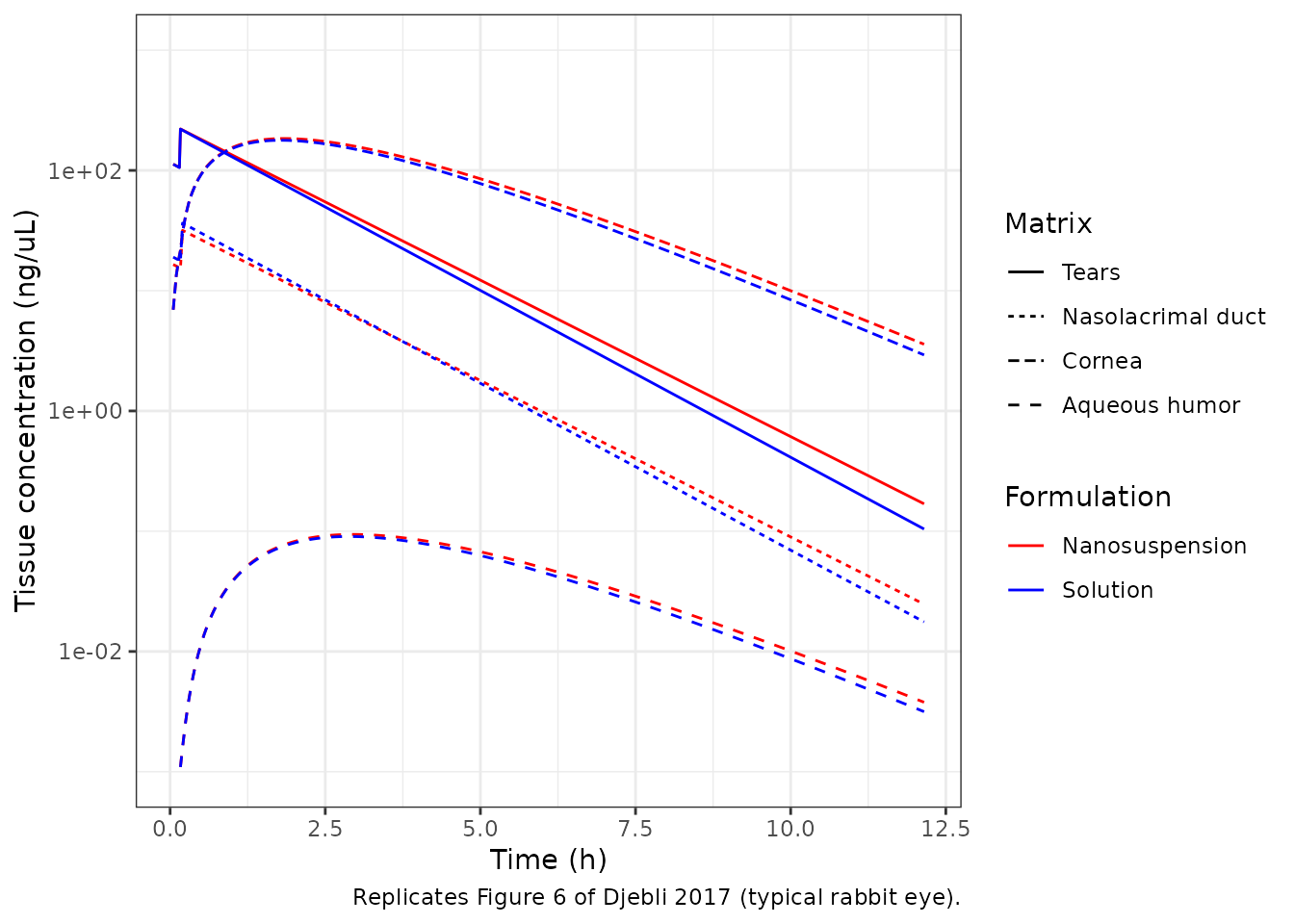
Comparison against Figure 6
Figure 6 of the paper is a raster image. The maintainers digitised it at seven times between 2 and 12 h (after the curves for the four matrices have separated), for both formulations. The axis calibration used the printed tick marks; the reading error is a few percent.
fig6 <- tibble::tribble(
  ~time, ~form, ~matrix, ~conc,
  1.998, 0L, "Ccornea", 169, 1.998, 0L, "Ctear", 66.8,
  1.998, 0L, "Cnasolacrimal_duct", 11.8, 1.998, 0L, "Caqueous_humour", 0.0755,
  2.985, 0L, "Ccornea", 145, 2.985, 0L, "Ctear", 36.1,
  2.985, 0L, "Cnasolacrimal_duct", 6.39, 2.985, 0L, "Caqueous_humour", 0.0858,
  3.997, 0L, "Ccornea", 109, 3.997, 0L, "Ctear", 19,
  3.997, 0L, "Cnasolacrimal_duct", 3.03, 3.997, 0L, "Caqueous_humour", 0.0777,
  5.995, 0L, "Ccornea", 51.6, 5.995, 0L, "Ctear", 5.3,
  5.995, 0L, "Cnasolacrimal_duct", 0.885, 5.995, 0L, "Caqueous_humour", 0.0451,
  7.994, 0L, "Ccornea", 21.6, 7.994, 0L, "Ctear", 1.48,
  7.994, 0L, "Cnasolacrimal_duct", 0.251, 7.994, 0L, "Caqueous_humour", 0.0211,
  9.992, 0L, "Ccornea", 8.5, 9.992, 0L, "Ctear", 0.421,
  9.992, 0L, "Cnasolacrimal_duct", 0.0713, 9.992, 0L, "Caqueous_humour", 0.00869,
  11.991, 0L, "Ccornea", 3.21, 11.991, 0L, "Ctear", 0.118,
  11.991, 0L, "Cnasolacrimal_duct", 0.0199, 11.991, 0L, "Caqueous_humour", 0.00343,
  1.998, 1L, "Ccornea", 179, 1.998, 1L, "Ctear", 72.8,
  1.998, 1L, "Cnasolacrimal_duct", 10.7, 1.998, 1L, "Caqueous_humour", 0.0811,
  2.985, 1L, "Ccornea", 158, 2.985, 1L, "Ctear", 41.1,
  2.985, 1L, "Cnasolacrimal_duct", 6.03, 2.985, 1L, "Caqueous_humour", 0.0935,
  3.997, 1L, "Ccornea", 120, 3.997, 1L, "Ctear", 22.2,
  3.997, 1L, "Cnasolacrimal_duct", 3.21, 3.997, 1L, "Caqueous_humour", 0.0846,
  5.995, 1L, "Ccornea", 57.9, 5.995, 1L, "Ctear", 6.76,
  5.995, 1L, "Cnasolacrimal_duct", 0.979, 5.995, 1L, "Caqueous_humour", 0.0498,
  7.994, 1L, "Ccornea", 24.9, 7.994, 1L, "Ctear", 2.03,
  7.994, 1L, "Cnasolacrimal_duct", 0.298, 7.994, 1L, "Caqueous_humour", 0.0237,
  9.992, 1L, "Ccornea", 10.1, 9.992, 1L, "Ctear", 0.628,
  9.992, 1L, "Cnasolacrimal_duct", 0.0922, 9.992, 1L, "Caqueous_humour", 0.0102,
  11.991, 1L, "Ccornea", 3.92, 11.991, 1L, "Ctear", 0.189,
  11.991, 1L, "Cnasolacrimal_duct", 0.0277, 11.991, 1L, "Caqueous_humour", 0.00413
)

# Solve the typical eye at the digitised times under two dosing readings:
# the protocol (two 60 ug drops 10 min apart) and a single 120 ug bolus.
predict_fig6 <- function(dose_rows) {
  out <- lapply(0:1, function(f) {
    ev <- bind_rows(
      mutate(dose_rows, id = 1L, evid = 1L, cmt = "tear", dvid = NA_integer_),
      tibble::tibble(id = 1L, time = unique(fig6$time), amt = 0, evid = 0L, cmt = "tear", dvid = 1L)
    ) |>
      arrange(time, desc(evid)) |>
      mutate(FORM_FV60165_NANOSUSP = f)
    rxode2::rxSolve(mod_typical, ev, returnType = "data.frame") |>
      select(time, all_of(names(matrix_label))) |>
      pivot_longer(-time, names_to = "matrix", values_to = "pred") |>
      mutate(form = f)
  })
  inner_join(fig6, bind_rows(out), by = c("time", "form", "matrix")) |>
    mutate(pct_diff = 100 * (pred - conc) / conc)
}

chk_split <- predict_fig6(tibble::tibble(time = drop_times, amt = dose_per_drop))
#> ℹ omega/sigma items treated as zero: 'etalfdepot', 'etalk_tear_nasolacrimal_duct', 'etalk_tear_cornea', 'etalq_cornea_aqueous_humour', 'etalcl_nasolacrimal_duct', 'etalcl_aqueous_humour', 'etalv_tear', 'etalv_nasolacrimal_duct', 'etalv_cornea', 'etalv_aqueous_humour'
#> ℹ omega/sigma items treated as zero: 'etalfdepot', 'etalk_tear_nasolacrimal_duct', 'etalk_tear_cornea', 'etalq_cornea_aqueous_humour', 'etalcl_nasolacrimal_duct', 'etalcl_aqueous_humour', 'etalv_tear', 'etalv_nasolacrimal_duct', 'etalv_cornea', 'etalv_aqueous_humour'
chk_single <- predict_fig6(tibble::tibble(time = 0, amt = 2 * dose_per_drop))
#> ℹ omega/sigma items treated as zero: 'etalfdepot', 'etalk_tear_nasolacrimal_duct', 'etalk_tear_cornea', 'etalq_cornea_aqueous_humour', 'etalcl_nasolacrimal_duct', 'etalcl_aqueous_humour', 'etalv_tear', 'etalv_nasolacrimal_duct', 'etalv_cornea', 'etalv_aqueous_humour'
#> ℹ omega/sigma items treated as zero: 'etalfdepot', 'etalk_tear_nasolacrimal_duct', 'etalk_tear_cornea', 'etalq_cornea_aqueous_humour', 'etalcl_nasolacrimal_duct', 'etalcl_aqueous_humour', 'etalv_tear', 'etalv_nasolacrimal_duct', 'etalv_cornea', 'etalv_aqueous_humour'

chk_split |>
  mutate(
    Formulation = formulation_label[as.character(form)],
    Matrix = matrix_label[matrix]
  ) |>
  group_by(Formulation, Matrix) |>
  summarise(
    median_pct = round(median(pct_diff), 1),
    max_abs_pct = round(max(abs(pct_diff)), 1),
    .groups = "drop"
  ) |>
  rename(
    "Median % difference" = median_pct,
    "Max |% difference|" = max_abs_pct
  ) |>
knitr::kable(caption = "Packaged model (typical eye, two 60 ug drops) versus digitised Figure 6, 2-12 h.")| Formulation | Matrix | Median % difference | Max |% difference| |
|---|---|---|---|
| Nanosuspension | Aqueous humor | 0.0 | 1.4 |
| Nanosuspension | Cornea | 0.2 | 2.5 |
| Nanosuspension | Nasolacrimal duct | 0.0 | 2.4 |
| Nanosuspension | Tears | -0.3 | 2.1 |
| Solution | Aqueous humor | 1.2 | 5.7 |
| Solution | Cornea | 1.0 | 4.6 |
| Solution | Nasolacrimal duct | -1.9 | 6.4 |
| Solution | Tears | 0.4 | 2.4 |
bind_rows(
  mutate(chk_split, dosing = "Two 60 ug drops, 10 min apart"),
  mutate(chk_single, dosing = "Single 120 ug bolus")
) |>
  group_by(dosing) |>
  summarise(
    median_pct = round(median(pct_diff), 2),
    p90_abs_pct = round(unname(quantile(abs(pct_diff), 0.9)), 2),
    .groups = "drop"
  ) |>
  rename(
    "Dosing reading" = dosing,
    "Median % difference" = median_pct,
    "90th percentile |% difference|" = p90_abs_pct
  ) |>
knitr::kable(caption = "The protocol dosing reproduces Figure 6; a single bolus of the same total is biased low.")| Dosing reading | Median % difference | 90th percentile |% difference| |
|---|---|---|
| Single 120 ug bolus | -4.28 | 7.16 |
| Two 60 ug drops, 10 min apart | 0.19 | 3.23 |
stopifnot(
  # A mis-transcribed rate, volume, F1 or dose moves every matrix by tens of
  # percent; digitisation error is a few percent.
  abs(median(chk_split$pct_diff)) < 2,
  quantile(abs(chk_split$pct_diff), 0.9) < 6,
  # The protocol dosing fits the figure better than one bolus of the same total.
  median(abs(chk_split$pct_diff)) < median(abs(chk_single$pct_diff))
)
Closed-form check of the tear compartment
The tear compartment receives only the bolus doses and loses drug by
two first-order routes, so its concentration has a closed form,
C(t) = 1000 * F1 * sum(D * exp(-(k12 + k13) * (t - t_dose))) / V1.
Both sides use the same parameters, so the difference is pure ODE-solver
error.
tear_cf <- typ_long |>
  filter(matrix == "Ctear", time > 0) |>
  mutate(
    k12 = ifelse(FORM_FV60165_NANOSUSP == 1, 0.259, 0.299),
    cf = 1000 * 0.300 * dose_per_drop / 155 *
      (exp(-(k12 + 0.340) * time) +
        ifelse(time >= drop_times[2], exp(-(k12 + 0.340) * (time - drop_times[2])), 0)),
    rel_err = abs(conc - cf) / cf
  )
max(tear_cf$rel_err)
#> [1] 1.408358e-07
stopifnot(max(tear_cf$rel_err) < 1e-4)
Virtual cohort and stochastic simulation
A cohort of 100 eyes per formulation is simulated with the paper’s inter- individual variability. The paper fitted every eye as one individual; eyes of the same rabbit are treated as independent here, as in the paper.
rxode2::rxSetSeed(20170128)
n_per_arm <- 100L
sto_times <- sort(unique(c(0, 0.083, 0.25, 0.5, 1, 2, 4, 8, seq(0, 12, by = 0.25))))
ev_sto <- bind_rows(
  make_events(seq_len(n_per_arm), 0L, sto_times),
  make_events(n_per_arm + seq_len(n_per_arm), 1L, sto_times)
)
sim_sto <- rxode2::rxSolve(
  mod,
  ev_sto,
  keep = "FORM_FV60165_NANOSUSP",
  returnType = "data.frame"
)
sto_long <- sim_sto |>
  select(id, time, FORM_FV60165_NANOSUSP, all_of(names(matrix_label))) |>
  pivot_longer(all_of(names(matrix_label)), names_to = "matrix", values_to = "conc") |>
  mutate(
    Formulation = formulation_label[as.character(FORM_FV60165_NANOSUSP)],
    Matrix = factor(matrix_label[matrix], levels = matrix_label)
  )
sto_long |>
  filter(time > 0) |>
  group_by(Matrix, time) |>
  summarise(
    p05 = quantile(conc, 0.05),
    p50 = median(conc),
    p95 = quantile(conc, 0.95),
    .groups = "drop"
  ) |>
  ggplot(aes(time, p50)) +
  geom_ribbon(aes(ymin = p05, ymax = p95), fill = "steelblue", alpha = 0.3) +
  geom_line() +
  facet_wrap(~Matrix, scales = "free_y") +
  scale_y_log10() +
  labs(
    x = "Time (h)",
    y = "Concentration (ng/uL)",
    caption = paste(
      "Median and 5th-95th percentiles, both formulations pooled.",
      "Compare with the prediction intervals of Figure 4 of Djebli 2017."
    )
  ) +
  theme_bw()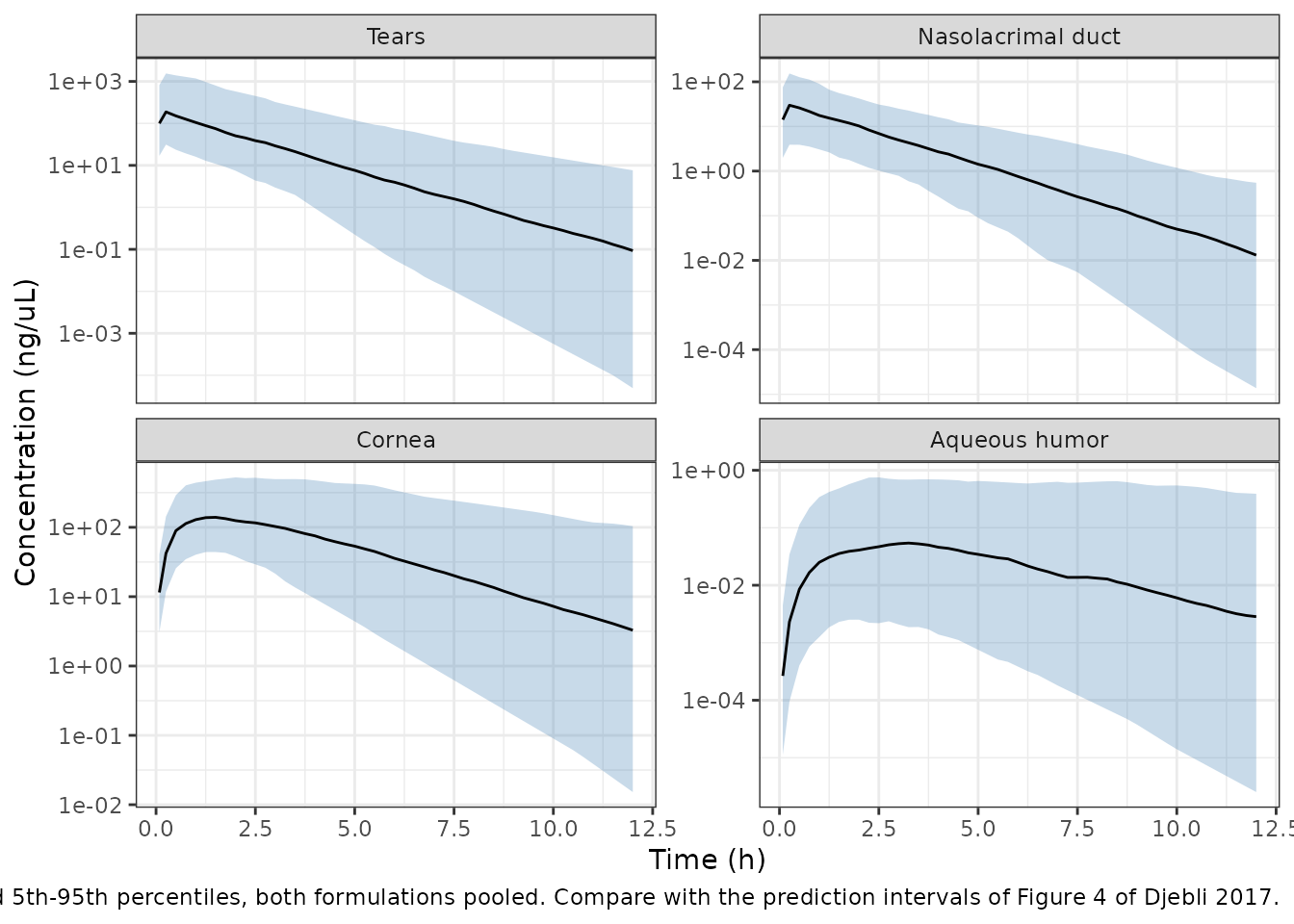
The observed concentrations spanned 0.0202 to 6260 ng/uL across the four matrices (Section 3); the simulated 5th-95th percentile bands cover the same orders of magnitude, with aqueous humor lowest and tears highest at early times, as in Figure 4.
PKNCA
Non-compartmental parameters over 0-12 h are computed for each formulation in the cornea (the target tissue) and the tears. The paper reports no NCA values, so the table is descriptive.
nca_conc <- sto_long |>
  filter(matrix %in% c("Ccornea", "Ctear"), !is.na(conc)) |>
  mutate(treatment = paste(Formulation, Matrix, sep = " / ")) |>
  select(id, time, conc, treatment)

nca_dose <- nca_conc |>
  distinct(id, treatment) |>
  tidyr::expand_grid(time = drop_times) |>
  mutate(amt = dose_per_drop)

conc_obj <- PKNCA::PKNCAconc(nca_conc, conc ~ time | treatment + id)
dose_obj <- PKNCA::PKNCAdose(nca_dose, amt ~ time | treatment + id)
intervals <- data.frame(
  start = 0,
  end = 12,
  cmax = TRUE,
  tmax = TRUE,
  auclast = TRUE
)
nca_res <- PKNCA::pk.nca(PKNCA::PKNCAdata(conc_obj, dose_obj, intervals = intervals))

as.data.frame(nca_res) |>
  filter(PPTESTCD %in% c("cmax", "tmax", "auclast")) |>
  group_by(treatment, PPTESTCD) |>
  summarise(median = signif(median(PPORRES), 3), .groups = "drop") |>
  pivot_wider(names_from = PPTESTCD, values_from = median) |>
  rename(
    "Formulation / matrix" = treatment,
    "Cmax (ng/uL)" = cmax,
    "Tmax (h)" = tmax,
    "AUC0-12 (h*ng/uL)" = auclast
  ) |>
knitr::kable(caption = "Median PKNCA parameters, 100 simulated eyes per formulation.")| Formulation / matrix | AUC0-12 (h*ng/uL) | Cmax (ng/uL) | Tmax (h) |
|---|---|---|---|
| Nanosuspension / Cornea | 646 | 157 | 1.75 |
| Nanosuspension / Tears | 280 | 186 | 0.25 |
| Solution / Cornea | 628 | 146 | 1.50 |
| Solution / Tears | 300 | 191 | 0.25 |
The typical-value cornea profile peaks at about 1.8 h, at 178 ng/uL for the solution and 184 ng/uL for the nanosuspension (Figure 6); the nanosuspension’s slower loss to the naso-lacrimal duct (k12 0.259 versus 0.299 1/h) leaves slightly more drug in the tears and cornea at late times.
cornea_peak <- typ_long |>
  filter(matrix == "Ccornea") |>
  group_by(Formulation) |>
  slice_max(conc, n = 1) |>
  ungroup()
cornea_peak |> select(Formulation, time, conc)
#> # A tibble: 2 × 3
#>   Formulation     time  conc
#>   <chr>          <dbl> <dbl>
#> 1 Nanosuspension  1.85  184.
#> 2 Solution        1.8   178.
stopifnot(
  all(abs(cornea_peak$time - 1.8) <= 0.1),
  abs(cornea_peak$conc[cornea_peak$Formulation == "Solution"] - 178) < 1,
  abs(cornea_peak$conc[cornea_peak$Formulation == "Nanosuspension"] - 184) < 1
)
Assumptions and deviations
- Dose entering the model. Section 2.5.2 states that one third of the instilled dose was entered into the analysis dataset, because at most 10 uL of each 30 uL drop stays in the tear film. The model is dosed with 60 ug of prodrug FV-80228 per drop, at 0 and 10 min. Dose amounts are prodrug mass, not FV-60165 molar equivalents (MW 554 vs 450): the comparison with Figure 6 above reproduces the published typical profiles with this reading, whereas a molar conversion would put every curve about 19% low. The relative bioavailability F1 absorbs both the prodrug-to-drug conversion and the loss from the eye surface.
-
Form of the inter-individual variability. The paper
selected a “proportional error model” for IIV,
P = TV * (1 + eta), and Table 1 prints100 * omegaas a CV%: the 95% confidence intervals printed for each CV are reproduced asCV * sqrt(1 +/- 1.96 * RSE)with the RSE on the variance, which fixes that scale. The proportional form cannot be simulated with these values: with a CV of 437% on V2,1 + etais negative, and so is the naso-lacrimal duct volume, in about 41% of eyes. The packaged model therefore uses log-normal IIV at the same CV,omega^2 = log((CV/100)^2 + 1)(for example 3.00 for V2 and 0.312 for F1). The typical-value profiles are unaffected; the spread of the stochastic cohort below is the log-normal one, not the paper’s. The paper reports high eta shrinkage on several of these parameters (for example 91.5% on k12 and 98.5% on V3), so the IIV is weakly informed by the data in either form. -
Residual error. The paper estimated one
proportional sigma (0.491%) for all four matrices. nlmixr2 needs a
separate residual parameter per endpoint, so the same value is carried
four times (
propSd_Ctear,propSd_Cnasolacrimal_duct,propSd_Ccornea,propSd_Caqueous_humour). A refit that wants the paper’s constraint must tie them. -
Formulation coding. The paper does not say which
formulation it coded as
- The two estimated k12 values are carried as separate parameters and
FORM_FV60165_NANOSUSP(1 = nanosuspension) only selects between them, so the choice of coding does not change any prediction. The IIV on k12 is shared by both formulations.
- The two estimated k12 values are carried as separate parameters and
-
Compartment names. The four states use the
library’s bare ocular-anatomy compartment names
tear,nasolacrimal_duct,corneaandaqueous_humour, registered with this model alongside the existingretinaandvitreous. The tear compartment’s matrix is recorded as tear fluid (collected on Schirmer strips); the duct and cornea were assayed as tissue homogenates. -
Bioavailability parameter. F1 is carried as
lfdepot, the library’s usual name for the bioavailability of the dosed compartment, and applied totear(the dose site) rather than to adepotstate. - Contralateral eyes. Both eyes of each rabbit were fitted as separate individuals with no shared random effect, and are simulated that way here.