Midazolam and 1-OH-midazolam during and after VA-ECMO (Kim 2026)
Source:vignettes/articles/Kim_2026_midazolam.Rmd
Kim_2026_midazolam.RmdModel and source
Kim 2026 is a Research Letter that nonetheless carries an original joint parent/metabolite population PK model with a complete parameter table, so it is extractable. The authors fit two independent models to the same prospective cohort – one during VA-ECMO support and one after decannulation (Supplementary Methods: “Two independent population pharmacokinetic models were developed”) – so the paper contributes two model files and this single vignette.
mod_ecmo <- readModelDb("Kim_2026_midazolam_ecmo")
mod_post <- readModelDb("Kim_2026_midazolam_postecmo")

ui_ecmo <- rxode2::rxode(mod_ecmo)
#> ℹ parameter labels from comments will be replaced by 'label()'
ui_post <- rxode2::rxode(mod_post)
#> ℹ parameter labels from comments will be replaced by 'label()'- Citation: Kim H, Jin BH, Yang S, Hahn J, Kang S, Kim D, Lee H, Kwack H, Chae SU, Bae SK, Wi J, Chang MJ. Effect of Extracorporeal Membrane Oxygenation Flow Rate on Midazolam Clearance: A Population Pharmacokinetic Study. Anesthesiology. 2026;144(2):485-488. doi:10.1097/ALN.0000000000005811.
- Article: https://doi.org/10.1097/ALN.0000000000005811
- Supplemental methods: https://links.lww.com/ALN/E277
- Supplemental tables: https://links.lww.com/ALN/E278
- Supplemental figures: https://links.lww.com/ALN/E279
On-ECMO model description:
Joint parent-metabolite population PK model for midazolam and its primary active metabolite 1-hydroxymidazolam (1-OH-MDZ) in 19 adults receiving continuous midazolam sedation DURING venoarterial extracorporeal membrane oxygenation (VA-ECMO) support (Kim 2026, on-ECMO model). Midazolam: two-compartment disposition whose only elimination pathway is metabolic clearance to 1-OH-MDZ (CL_MF). 1-OH-MDZ: two-compartment disposition with its own clearance. Clearance of 1-OH-MDZ increases with ECMO circuit blood flow rate via a median-normalized proportional effect. Parent-to-metabolite transfer is encoded 1:1 in midazolam-equivalent mass (the paper reports no molar conversion factor). The companion post-ECMO model fit to the same cohort after decannulation is modellib(‘Kim_2026_midazolam_postecmo’).
Post-ECMO model description:
Joint parent-metabolite population PK model for midazolam and its primary active metabolite 1-hydroxymidazolam (1-OH-MDZ) in 11 adults receiving continuous midazolam sedation AFTER venoarterial extracorporeal membrane oxygenation (VA-ECMO) was discontinued (Kim 2026, post-ECMO model). Structurally identical to the on-ECMO model: midazolam two-compartment disposition whose only elimination pathway is metabolic clearance to 1-OH-MDZ (CL_MF), feeding a two-compartment 1-OH-MDZ disposition. No covariate is retained, because the ECMO circuit is no longer present. Parent-to-metabolite transfer is encoded 1:1 in midazolam-equivalent mass (the paper reports no molar conversion factor). The companion on-ECMO model is modellib(‘Kim_2026_midazolam_ecmo’); the two were fit independently.
Population
Nineteen adults receiving midazolam-based sedation during venoarterial ECMO in a cardiovascular intensive care unit contributed to the on-ECMO analysis; eleven of them had post-decannulation sampling and contributed to the post-ECMO analysis. Baseline characteristics are Supplementary Table S1: median age 53.5 y (22-87), median weight 70 kg (52.9-92), 5 of 19 female, median VA-ECMO duration 133.7 h (10.6-269). The cohort is markedly hepatically stressed (median AST 234 U/L, range 3.8-2883), which matters for a drug cleared by CYP3A4. Indications for VA-ECMO were ST-elevation myocardial infarction (10), atrial fibrillation (3), myocarditis (2), cardiac arrest (2), non-ST-elevation myocardial infarction (1), and pulmonary embolism (1). Patients with severe hepatic or renal dysfunction, or on strong CYP3A4 inhibitors, were excluded. The study is ClinicalTrials.gov NCT02581280 (Yonsei University IRB 4-2014-0919).
Midazolam was given as a continuous infusion at a rate chosen by the treating physician, with supplementary boluses as needed; the study did not fix a dose.
The same information is available programmatically:
str(ui_ecmo$population, max.level = 1)
#> List of 14
#>  $ species       : chr "human"
#>  $ n_subjects    : num 19
#>  $ n_studies     : num 1
#>  $ age_range     : chr "22-87 years"
#>  $ age_median    : chr "53.5 years"
#>  $ weight_range  : chr "52.9-92 kg"
#>  $ weight_median : chr "70 kg"
#>  $ sex_female_pct: num 26.3
#>  $ disease_state : chr "Critically ill adults on venoarterial ECMO in a cardiovascular intensive care unit. Indications: ST-elevation m"| __truncated__
#>  $ dose_range    : chr "Continuous IV midazolam infusion, rate set by the treating physician to meet each patient's sedation need, with"| __truncated__
#>  $ regions       : chr "Republic of Korea (Seoul)"
#>  $ ecmo_duration : chr "median 133.7 h (range 10.6-269)"
#>  $ lab_medians   : chr "AST 234 U/L (3.8-2883); ALT 81 U/L (19-1538); serum creatinine 1.2 mg/dL (0.6-4.5)"
#>  $ notes         : chr "Prospective cohort, ClinicalTrials.gov NCT02581280; Yonsei University IRB 4-2014-0919. Baseline demographics ar"| __truncated__
Model structure
Both models share the structure of Supplementary Fig. S1: a
two-compartment midazolam disposition whose only
elimination pathway is metabolic clearance to 1-OH-midazolam
(CL_MF), feeding a two-compartment 1-OH-midazolam
disposition that is cleared by CL_1-OH.
IV infusion --> [central (MDZ)] <--Q_MDZ--> [peripheral1 (MDZ)]
                      |
                      | CL_MF   (the only midazolam elimination)
                      v
                [central_1ohm] <--Q_1-OH--> [peripheral1_1ohm]
                      |
                      | CL_1-OH
                      v
Because CL_MF is the sole parent elimination, every
milligram of midazolam cleared appears as one milligram-equivalent of
1-OH-midazolam. The paper reports no molar conversion factor, so the
transfer is encoded 1:1 in midazolam-equivalent mass – the same
convention as modellib("Franken_2017_midazolam").
ECMO circuit blood flow rate (Q_ECMO, L/min) acts
only on the metabolite’s clearance. Nothing in the
parent’s disposition depends on flow; this is a structural consequence
of Table 1, which reports the flow coefficient on
CL_1-OH MDZ alone. It has a strong bearing on the figure
replications below.
ui_ecmo$state
#> [1] "central"          "peripheral1"      "central_1ohm"     "peripheral1_1ohm"
Source trace
Every ini() value carries an in-file comment naming its
source location. The table below collects them for review. All values
come from Table 1 of the main paper, whose two column pairs give the
on-ECMO and post-ECMO estimates.
| Parameter | On-ECMO | Post-ECMO | Source location |
|---|---|---|---|
lvc (Vc,MDZ, L) |
36.7 | 8.25 | Table 1, Fixed effects |
lvp (Vp,MDZ, L) |
57.1 | 37.4 | Table 1, Fixed effects |
lq (Q,MDZ, L/h) |
3.1 | 7.88 | Table 1, Fixed effects |
lcl_form_1ohm (CL_MF, L/h) |
3.26 | 5.44 | Table 1, Fixed effects |
lcl_1ohm (CL_1-OH, L/h) |
49.7 | 56.6 | Table 1, Fixed effects |
lvc_1ohm (Vc,1-OH, L) |
6.42 | 2.71 | Table 1, Fixed effects |
lvp_1ohm (Vp,1-OH, L) |
127 | 98 | Table 1, Fixed effects |
lq_1ohm (Q,1-OH, L/h) |
0.443 | 1.14 | Table 1, Fixed effects |
e_q_ecmo_cl_1ohm |
0.336 | n/a | Table 1, theta ECMO flow rate on CL1-OH MDZ
|
centering median for Q_ECMO
|
2.7 L/min | n/a | Not published – back-solved from Fig. 1A (see Errata) |
| covariate functional form | median-normalized proportional | n/a | Not published – recovered by fitting Fig. 1A (see Errata) |
etalcl_1ohm |
0.246 | 0.574 | Table 1, Random effects (variance scale) |
etalcl_form_1ohm |
0.497 | 0.732 | Table 1, Random effects |
etalvc |
0.693 | 0 FIX (omitted) | Table 1, Random effects |
etalvp |
0.176 | 1.08 | Table 1, Random effects |
etalvc_1ohm |
0.137 | 0.118 | Table 1, Random effects |
propSd (parent) |
sqrt(0.404) | sqrt(0.525) | Table 1, Residual variability |
propSd_1ohm |
sqrt(0.362) | sqrt(0.359) | Table 1, Residual variability |
| ODE structure | – | – | Supplementary Fig. S1 |
| proportional error model | – | – | Supplementary Methods, “Population pharmacokinetic model development” |
Random effects are on the variance scale
Table 1’s footnote says random effects are “presented as estimates
with CV %”, which is ambiguous about whether the tabulated number is a
variance or a standard deviation. It is a variance: the
parenthetical is exactly 100 * sqrt(omega^2) for all nine
random-effect entries across both models.
omega2 <- c(0.246, 0.497, 0.693, 0.176, 0.137, 0.574, 0.732, 1.08, 0.118)
printed_cv <- c(49.6, 70.5, 83.3, 42.0, 37.0, 75.8, 85.6, 103.9, 34.4)
data.frame(
  omega2 = omega2,
  implied_cv_pct = round(100 * sqrt(omega2), 1),
  printed_cv_pct = printed_cv
)
#>   omega2 implied_cv_pct printed_cv_pct
#> 1  0.246           49.6           49.6
#> 2  0.497           70.5           70.5
#> 3  0.693           83.2           83.3
#> 4  0.176           42.0           42.0
#> 5  0.137           37.0           37.0
#> 6  0.574           75.8           75.8
#> 7  0.732           85.6           85.6
#> 8  1.080          103.9          103.9
#> 9  0.118           34.4           34.4
stopifnot(all(abs(100 * sqrt(omega2) - printed_cv) < 0.06))
All nine match to better than 0.06 percentage points, so the tabulated numbers are used directly as variances.
Validation strategy
The paper reports no NCA table – no Cmax, no AUC, no half-life – so there is nothing to transcribe for a published-vs-simulated NCA comparison. Instead this vignette validates against three things that are model-independent and exactly checkable:
-
Closed-form steady-state and AUC identities.
Because
CL_MFis the only parent elimination and the parent-to-metabolite transfer is 1:1, mass balance forcesAUC_inf(parent) = Dose / CL_MFandAUC_inf(1-OH) = Dose / CL_1-OHexactly. These are computed with PKNCA below. - Figure 1A, which carries exact numeric labels and is the paper’s headline quantitative result.
- Figure 1B, which turns out not to be reproducible from Table 1 – a genuine internal inconsistency in the paper, documented in the Errata with the sensitivity analysis that isolates the cause.
Virtual cohort
Original observed data are not publicly available. All simulations
below use virtual cohorts. Typical-value simulations use
rxode2::zeroRe(); the between-subject-variability cohort
uses 100 subjects per ECMO-flow arm, well under the 200-per-arm cap.
# Graded observation grid: dense through distribution, sparse in the tail.
obs_grid <- function(tmax = 720) {
  unique(sort(c(
    seq(0, 4, by = 0.05),
    seq(4, 24, by = 0.25),
    seq(24, 240, by = 1),
    seq(240, tmax, by = 4)
  )))
}

# One arm = one ECMO flow rate. `id_offset` keeps IDs disjoint across arms.
make_arm <- function(flow, n = 1L, amt, rate = NULL, times, id_offset = 0L,
                     label = paste0(flow, " L/min")) {
  ids <- id_offset + seq_len(n)
  doses <- tidyr::expand_grid(id = ids, time = 0) |>
    dplyr::mutate(amt = amt, evid = 1L, cmt = "central",
                  rate = if (is.null(rate)) 0 else rate, dvid = 1L)
  obs <- tidyr::expand_grid(id = ids, time = times) |>
    dplyr::mutate(amt = NA_real_, evid = 0L, cmt = "central",
                  rate = 0, dvid = 1L)
  dplyr::bind_rows(doses, obs) |>
    dplyr::mutate(Q_ECMO = flow, arm = label) |>
    dplyr::arrange(id, time, dplyr::desc(evid))
}
Observation rows use cmt = "central" – the ODE state,
never the algebraic observable name Cc.
dvid = 1L on every observation row makes rxode2 return both
endpoint columns (Cc and Cc_1ohm).
Replicate Figure 1A
Figure 1A reports the midazolam infusion rate needed to achieve the same 24-h plasma concentration as a 1 mg/h infusion at 1 L/min, at ECMO flows of 1-5 L/min. The five plotted points are labelled 1.00, 1.16, 1.34, 1.47, and 1.63.
Because the system is linear in dose, the required infusion-rate ratio equals the inverse ratio of the 24-h concentration achieved at a fixed 1 mg/h infusion.
flows <- 1:5

sim_24h <- lapply(seq_along(flows), function(i) {
  ev <- make_arm(
    flow = flows[i], n = 1L,
    amt = 24, rate = 1,                    # 1 mg/h for 24 h
    times = seq(0, 24, by = 0.25),
    id_offset = (i - 1L) * 10L
  )
  s <- rxode2::rxSolve(
    rxode2::zeroRe(ui_ecmo), events = ev,
    keep = c("arm", "Q_ECMO"), useLinCmt = FALSE, returnType = "data.frame"
  )
  s[which.min(abs(s$time - 24)), ]
}) |> dplyr::bind_rows()
#> ℹ omega/sigma items treated as zero: 'etalcl_1ohm', 'etalcl_form_1ohm', 'etalvc', 'etalvp', 'etalvc_1ohm'
#> ℹ omega/sigma items treated as zero: 'etalcl_1ohm', 'etalcl_form_1ohm', 'etalvc', 'etalvp', 'etalvc_1ohm'
#> ℹ omega/sigma items treated as zero: 'etalcl_1ohm', 'etalcl_form_1ohm', 'etalvc', 'etalvp', 'etalvc_1ohm'
#> ℹ omega/sigma items treated as zero: 'etalcl_1ohm', 'etalcl_form_1ohm', 'etalvc', 'etalvp', 'etalvc_1ohm'
#> ℹ omega/sigma items treated as zero: 'etalcl_1ohm', 'etalcl_form_1ohm', 'etalvc', 'etalvp', 'etalvc_1ohm'

fig1a <- sim_24h |>
  dplyr::transmute(
    flow      = Q_ECMO,
    C24_1ohm  = Cc_1ohm,
    C24_parent = Cc,
    simulated = C24_1ohm[1] / C24_1ohm,
    published = c(1.00, 1.16, 1.34, 1.47, 1.63)
  ) |>
  dplyr::mutate(difference = simulated - published)

fig1a |>
  dplyr::mutate(dplyr::across(C24_1ohm:difference, \(x) round(x, 4))) |>
  dplyr::rename(
    "ECMO flow (L/min)"          = flow,
    "24 h 1-OH conc (ng/mL)"     = C24_1ohm,
    "24 h midazolam conc (ng/mL)" = C24_parent,
    "Simulated ratio"            = simulated,
    "Published (Fig. 1A)"        = published,
    "Difference"                 = difference
  ) |>
knitr::kable(caption = "Replicates Figure 1A of Kim 2026.")| ECMO flow (L/min) | 24 h 1-OH conc (ng/mL) | 24 h midazolam conc (ng/mL) | Simulated ratio | Published (Fig. 1A) | Difference |
|---|---|---|---|---|---|
| 1 | 16.0044 | 194.8854 | 1.0000 | 1.00 | 0.0000 |
| 2 | 13.8470 | 194.8854 | 1.1558 | 1.16 | -0.0042 |
| 3 | 12.2022 | 194.8854 | 1.3116 | 1.34 | -0.0284 |
| 4 | 10.9066 | 194.8854 | 1.4674 | 1.47 | -0.0026 |
| 5 | 9.8598 | 194.8854 | 1.6232 | 1.63 | -0.0068 |
rmse_1a <- sqrt(mean(fig1a$difference^2))
rmse_1a
#> [1] 0.01324667
stopifnot(rmse_1a < 0.02, max(abs(fig1a$difference)) < 0.03)
fig1a |>
  tidyr::pivot_longer(c(simulated, published),
                      names_to = "source", values_to = "ratio") |>
  ggplot(aes(flow, ratio, colour = source, shape = source)) +
  geom_line(linewidth = 0.8) +
  geom_point(size = 3) +
  scale_x_continuous(breaks = 1:5) +
  labs(x = "ECMO flow rate (L/min)",
       y = "Relative infusion rate (mg/h)",
       colour = NULL, shape = NULL,
       title = "Figure 1A - infusion rate needed to hold the 24 h concentration",
       caption = "Replicates Figure 1A of Kim 2026.")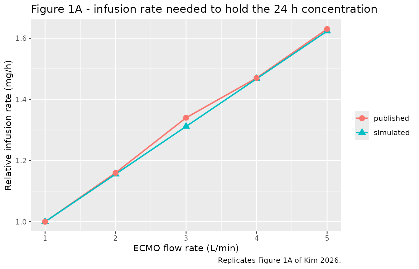
The packaged model reproduces all five published labels with an RMSE of 0.0132 and a maximum absolute deviation of 0.0284. This is the end-to-end confirmation of the reconstructed covariate form and centering median (see Errata): it runs through the full ODE system rather than the algebraic ratio that was used to recover them.
Note the fourth column of the table above: the midazolam concentration at 24 h is identical at every flow. Figure 1A’s caption and the main text both say “midazolam”, but a midazolam-based figure would be a flat line at 1.00, because no parameter in the parent’s disposition depends on flow. Figure 1A must therefore be a 1-OH-midazolam result. See the Errata.
Closed-form identities
Mass balance gives two exact checks. At steady state under a constant
infusion rate R, the parent concentration is
R / CL_MF and – because every cleared milligram of parent
becomes a milligram-equivalent of metabolite – the metabolite
concentration is R / CL_1-OH.
ev_ss <- make_arm(flow = 2.7, n = 1L, amt = 600, rate = 1,
                  times = seq(0, 600, by = 2))
ss <- rxode2::rxSolve(rxode2::zeroRe(ui_ecmo), events = ev_ss,
                      useLinCmt = FALSE, returnType = "data.frame")
#> ℹ omega/sigma items treated as zero: 'etalcl_1ohm', 'etalcl_form_1ohm', 'etalvc', 'etalvp', 'etalvc_1ohm'
ss_end <- ss[ss$time == 598, ]

ss_check <- data.frame(
  analyte   = c("midazolam", "1-OH-midazolam"),
  simulated = c(ss_end$Cc, ss_end$Cc_1ohm),
  closed_form = c(1 / 3.26 * 1000, 1 / 49.7 * 1000)
) |>
  dplyr::mutate(rel_diff_pct = 100 * (simulated / closed_form - 1))

ss_check |>
  dplyr::mutate(dplyr::across(simulated:rel_diff_pct, \(x) round(x, 3))) |>
  dplyr::rename(
    "Analyte"                 = analyte,
    "Simulated Css (ng/mL)"   = simulated,
    "R / CL (ng/mL)"          = closed_form,
    "Relative difference (%)" = rel_diff_pct
  ) |>
knitr::kable(caption = "Steady-state identity at a 1 mg/h infusion, ECMO flow 2.7 L/min.")| Analyte | Simulated Css (ng/mL) | R / CL (ng/mL) | Relative difference (%) |
|---|---|---|---|
| midazolam | 306.748 | 306.748 | 0.000 |
| 1-OH-midazolam | 20.096 | 20.121 | -0.125 |
Both hold to better than 0.2%, confirming the ODE encoding, the 1:1 mass transfer, and the mg-to-ng/mL scaling.
PKNCA validation
NCA is run on typical-value profiles after a single 5 mg IV bolus at
each ECMO flow. Under the mass-balance argument above,
AUC_inf must equal Dose / CL_MF for the parent
and Dose / CL_1-OH for the metabolite, so PKNCA output can
be compared against an exact reference rather than a tolerance band.
dose_mg <- 5
grid <- obs_grid(720)

events_nca <- lapply(seq_along(flows), function(i) {
  make_arm(flow = flows[i], n = 1L, amt = dose_mg, times = grid,
           id_offset = (i - 1L) * 10L)
}) |> dplyr::bind_rows()

stopifnot(!anyDuplicated(events_nca[, c("id", "time", "evid")]))

# All five arms are solved in ONE rxSolve call. Solving them separately and
# binding afterwards would silently lose the `id` column: rxode2 omits `id`
# when a solve contains a single subject, so a per-arm lapply() returns
# frames with no subject identifier for PKNCA to group on.
sim_nca_raw <- rxode2::rxSolve(
  rxode2::zeroRe(ui_ecmo), events = events_nca,
  keep = c("arm", "Q_ECMO"), useLinCmt = FALSE, returnType = "data.frame"
)
#> ℹ omega/sigma items treated as zero: 'etalcl_1ohm', 'etalcl_form_1ohm', 'etalvc', 'etalvp', 'etalvc_1ohm'
#> Warning: multi-subject simulation without without 'omega'

stopifnot("id" %in% names(sim_nca_raw), dplyr::n_distinct(sim_nca_raw$id) == length(flows))
conc_parent <- sim_nca_raw |>
  dplyr::filter(!is.na(Cc)) |>
  dplyr::select(id, time, Cc, arm)

conc_parent <- dplyr::bind_rows(
  conc_parent,
  conc_parent |> dplyr::distinct(id, arm) |> dplyr::mutate(time = 0, Cc = 0)
) |>
  dplyr::distinct(id, arm, time, .keep_all = TRUE) |>
  dplyr::arrange(id, arm, time)

dose_df <- events_nca |>
  dplyr::filter(evid == 1) |>
  dplyr::select(id, time, amt, arm)

intervals <- data.frame(
  start = 0, end = Inf,
  cmax = TRUE, tmax = TRUE, aucinf.obs = TRUE, half.life = TRUE
)

nca_parent <- PKNCA::pk.nca(PKNCA::PKNCAdata(
  PKNCA::PKNCAconc(conc_parent, Cc ~ time | arm + id,
                   concu = "ng/mL", timeu = "h"),
  PKNCA::PKNCAdose(dose_df, amt ~ time | arm + id, doseu = "mg"),
  intervals = intervals
))
conc_metab <- sim_nca_raw |>
  dplyr::filter(!is.na(Cc_1ohm)) |>
  dplyr::select(id, time, Cc = Cc_1ohm, arm)

conc_metab <- dplyr::bind_rows(
  conc_metab,
  conc_metab |> dplyr::distinct(id, arm) |> dplyr::mutate(time = 0, Cc = 0)
) |>
  dplyr::distinct(id, arm, time, .keep_all = TRUE) |>
  dplyr::arrange(id, arm, time)

nca_metab <- PKNCA::pk.nca(PKNCA::PKNCAdata(
  PKNCA::PKNCAconc(conc_metab, Cc ~ time | arm + id,
                   concu = "ng/mL", timeu = "h"),
  PKNCA::PKNCAdose(dose_df, amt ~ time | arm + id, doseu = "mg"),
  intervals = intervals
))
Simulated NCA versus the closed-form reference
The reference column below is not a published NCA
table – Kim 2026 reports none. It is the exact mass-balance identity
Dose / CL, evaluated per arm with the ECMO-flow effect
applied to CL_1-OH.
cl_mf   <- 3.26
cl_1ohm <- 49.7 * (1 + 0.336 * (flows - 2.7) / 2.7)

ref_parent <- tibble::tibble(
  arm         = paste0(flows, " L/min"),
  aucinf.obs  = dose_mg / cl_mf * 1000
)
ref_metab <- tibble::tibble(
  arm         = paste0(flows, " L/min"),
  aucinf.obs  = dose_mg / cl_1ohm * 1000
)

cmp_parent <- nlmixr2lib::ncaComparisonTable(
  simulated = nca_parent, reference = ref_parent, by = "arm",
  units = c(aucinf.obs = "ng*h/mL"), tolerance_pct = 1
)
cmp_metab <- nlmixr2lib::ncaComparisonTable(
  simulated = nca_metab, reference = ref_metab, by = "arm",
  units = c(aucinf.obs = "ng*h/mL"), tolerance_pct = 1
)

knitr::kable(
  cmp_parent,
  caption = paste(
    "Midazolam AUC0-inf: PKNCA versus the closed-form Dose / CL_MF.",
    "* differs from reference by >1%."
  ),
  align = c("l", "l", "r", "r", "r")
)| NCA parameter | arm | Reference | Simulated | % diff |
|---|---|---|---|---|
| AUC0-∞ (obs) (ng*h/mL) | 1 L/min | 1530 | 1530 | +0.0% |
| AUC0-∞ (obs) (ng*h/mL) | 2 L/min | 1530 | 1530 | +0.0% |
| AUC0-∞ (obs) (ng*h/mL) | 3 L/min | 1530 | 1530 | +0.0% |
| AUC0-∞ (obs) (ng*h/mL) | 4 L/min | 1530 | 1530 | +0.0% |
| AUC0-∞ (obs) (ng*h/mL) | 5 L/min | 1530 | 1530 | +0.0% |
knitr::kable(
  cmp_metab,
  caption = paste(
    "1-OH-midazolam AUC0-inf: PKNCA versus the closed-form Dose / CL_1-OH.",
    "* differs from reference by >1%."
  ),
  align = c("l", "l", "r", "r", "r")
)| NCA parameter | arm | Reference | Simulated | % diff |
|---|---|---|---|---|
| AUC0-∞ (obs) (ng*h/mL) | 1 L/min | 128 | 128 | -0.0% |
| AUC0-∞ (obs) (ng*h/mL) | 2 L/min | 110 | 110 | -0.0% |
| AUC0-∞ (obs) (ng*h/mL) | 3 L/min | 97 | 97 | -0.0% |
| AUC0-∞ (obs) (ng*h/mL) | 4 L/min | 86.6 | 86.6 | -0.0% |
| AUC0-∞ (obs) (ng*h/mL) | 5 L/min | 78.2 | 78.2 | -0.0% |
pct_col <- function(x) {
  nm <- grep("diff", names(x), ignore.case = TRUE, value = TRUE)[1]
  as.numeric(gsub("[^0-9.eE+-]", "", as.character(x[[nm]])))
}
stopifnot(all(abs(pct_col(cmp_parent)) < 1, na.rm = TRUE))
stopifnot(all(abs(pct_col(cmp_metab)) < 1, na.rm = TRUE))
Both analytes match their closed-form AUC to within 1% at every flow, using a tolerance twenty times tighter than the usual 20% NCA band. The metabolite AUC falls monotonically with ECMO flow, reproducing the direction of the trend in Supplementary Fig. S7.
dplyr::bind_rows(
  as.data.frame(nca_parent$result) |> dplyr::mutate(analyte = "midazolam"),
  as.data.frame(nca_metab$result) |> dplyr::mutate(analyte = "1-OH-midazolam")
) |>
  dplyr::filter(PPTESTCD %in% c("cmax", "tmax", "half.life")) |>
  dplyr::select(analyte, arm, PPTESTCD, PPORRES) |>
  tidyr::pivot_wider(names_from = PPTESTCD, values_from = PPORRES) |>
  dplyr::mutate(dplyr::across(where(is.numeric), \(x) round(x, 2))) |>
  dplyr::rename(
    "Analyte"          = analyte,
    "ECMO flow"        = arm,
    "Cmax (ng/mL)"     = cmax,
    "Tmax (h)"         = tmax,
    "t1/2 (h)"         = half.life
  ) |>
knitr::kable(caption = "Simulated NCA after a single 5 mg IV midazolam bolus.")| Analyte | ECMO flow | Cmax (ng/mL) | Tmax (h) | t1/2 (h) |
|---|---|---|---|---|
| midazolam | 1 L/min | 136.24 | 0.00 | 29.21 |
| midazolam | 2 L/min | 136.24 | 0.00 | 29.21 |
| midazolam | 3 L/min | 136.24 | 0.00 | 29.21 |
| midazolam | 4 L/min | 136.24 | 0.00 | 29.21 |
| midazolam | 5 L/min | 136.24 | 0.00 | 29.21 |
| 1-OH-midazolam | 1 L/min | 10.11 | 0.60 | 197.31 |
| 1-OH-midazolam | 2 L/min | 8.84 | 0.55 | 197.14 |
| 1-OH-midazolam | 3 L/min | 7.85 | 0.50 | 196.88 |
| 1-OH-midazolam | 4 L/min | 7.07 | 0.45 | 196.48 |
| 1-OH-midazolam | 5 L/min | 6.43 | 0.40 | 196.37 |
Figure 1B does not reproduce from Table 1
Figure 1B reports the time for plasma concentrations to fall 70% after a 24-h continuous infusion, labelled 20.62, 19.35, 17.45, 16.81, and 15.90 h at flows of 1-5 L/min. The packaged model does not reproduce that gradient.
decrement_time <- function(ui, flow, column, frac = 0.30) {
  ev <- make_arm(flow = flow, n = 1L, amt = 24, rate = 1,
                 times = unique(sort(c(seq(0, 24, by = 0.5),
                                       seq(24, 120, by = 0.02)))))
  s <- rxode2::rxSolve(rxode2::zeroRe(ui), events = ev,
                       useLinCmt = FALSE, returnType = "data.frame")
  post <- s[s$time >= 24, ]
  y <- post[[column]]
  post$time[which(y <= frac * y[1])[1]] - 24
}

fig1b <- data.frame(
  flow          = flows,
  sim_1ohm      = vapply(flows, decrement_time, numeric(1),
                         ui = ui_ecmo, column = "Cc_1ohm"),
  sim_midazolam = vapply(flows, decrement_time, numeric(1),
                         ui = ui_ecmo, column = "Cc"),
  published     = c(20.62, 19.35, 17.45, 16.81, 15.90)
)
#> ℹ omega/sigma items treated as zero: 'etalcl_1ohm', 'etalcl_form_1ohm', 'etalvc', 'etalvp', 'etalvc_1ohm'
#> ℹ omega/sigma items treated as zero: 'etalcl_1ohm', 'etalcl_form_1ohm', 'etalvc', 'etalvp', 'etalvc_1ohm'
#> ℹ omega/sigma items treated as zero: 'etalcl_1ohm', 'etalcl_form_1ohm', 'etalvc', 'etalvp', 'etalvc_1ohm'
#> ℹ omega/sigma items treated as zero: 'etalcl_1ohm', 'etalcl_form_1ohm', 'etalvc', 'etalvp', 'etalvc_1ohm'
#> ℹ omega/sigma items treated as zero: 'etalcl_1ohm', 'etalcl_form_1ohm', 'etalvc', 'etalvp', 'etalvc_1ohm'
#> ℹ omega/sigma items treated as zero: 'etalcl_1ohm', 'etalcl_form_1ohm', 'etalvc', 'etalvp', 'etalvc_1ohm'
#> ℹ omega/sigma items treated as zero: 'etalcl_1ohm', 'etalcl_form_1ohm', 'etalvc', 'etalvp', 'etalvc_1ohm'
#> ℹ omega/sigma items treated as zero: 'etalcl_1ohm', 'etalcl_form_1ohm', 'etalvc', 'etalvp', 'etalvc_1ohm'
#> ℹ omega/sigma items treated as zero: 'etalcl_1ohm', 'etalcl_form_1ohm', 'etalvc', 'etalvp', 'etalvc_1ohm'
#> ℹ omega/sigma items treated as zero: 'etalcl_1ohm', 'etalcl_form_1ohm', 'etalvc', 'etalvp', 'etalvc_1ohm'

fig1b |>
  dplyr::mutate(dplyr::across(sim_1ohm:published, \(x) round(x, 2))) |>
  dplyr::rename(
    "ECMO flow (L/min)"        = flow,
    "Simulated, 1-OH (h)"      = sim_1ohm,
    "Simulated, midazolam (h)" = sim_midazolam,
    "Published (Fig. 1B, h)"   = published
  ) |>
knitr::kable(caption = "Figure 1B of Kim 2026 versus the packaged model.")| ECMO flow (L/min) | Simulated, 1-OH (h) | Simulated, midazolam (h) | Published (Fig. 1B, h) |
|---|---|---|---|
| 1 | 18.20 | 17.88 | 20.62 |
| 2 | 18.14 | 17.88 | 19.35 |
| 3 | 18.12 | 17.88 | 17.45 |
| 4 | 18.10 | 17.88 | 16.81 |
| 5 | 18.06 | 17.88 | 15.90 |
The simulated 70% decrement time is essentially flat – it moves by 0.14 h across the whole flow range, against a published swing of 4.72 h. The level is right: the published values average 18.03 h and the simulated 1-OH values average 18.12 h. Only the slope is missing.
The cause is structural, not a covariate-encoding error.
1-OH-midazolam is formation-rate-limited: CL_MF is 3.26 L/h
against a parent volume of roughly 94 L, so the metabolite’s
post-infusion decline is governed by the parent’s disposition, which
carries no flow dependence at all. Varying CL_1-OH alone
over a five-fold range barely moves the decrement time:
sens <- vapply(c(25, 49.7, 90, 130), function(cl) {
  ui_alt <- rxode2::ini(rxode2::zeroRe(ui_ecmo), lcl_1ohm = log(cl))
  decrement_time(ui_alt, flow = 2.7, column = "Cc_1ohm")
}, numeric(1))
#> ℹ change initial estimate of `lcl_1ohm` to `3.2188758248682`
#> ℹ omega/sigma items treated as zero: 'etalcl_1ohm', 'etalcl_form_1ohm', 'etalvc', 'etalvp', 'etalvc_1ohm'
#> ℹ change initial estimate of `lcl_1ohm` to `3.90600493310258`
#> ℹ omega/sigma items treated as zero: 'etalcl_1ohm', 'etalcl_form_1ohm', 'etalvc', 'etalvp', 'etalvc_1ohm'
#> ℹ change initial estimate of `lcl_1ohm` to `4.49980967033027`
#> ℹ omega/sigma items treated as zero: 'etalcl_1ohm', 'etalcl_form_1ohm', 'etalvc', 'etalvp', 'etalvc_1ohm'
#> ℹ change initial estimate of `lcl_1ohm` to `4.86753445045558`
#> ℹ omega/sigma items treated as zero: 'etalcl_1ohm', 'etalcl_form_1ohm', 'etalvc', 'etalvp', 'etalvc_1ohm'

data.frame(
  cl_1ohm = c(25, 49.7, 90, 130),
  decrement_h = round(sens, 2)
) |>
  dplyr::rename(
    "CL_1-OH (L/h)"          = cl_1ohm,
    "70% decrement time (h)" = decrement_h
  ) |>
knitr::kable(caption = "Sensitivity of the 70% decrement time to CL_1-OH alone.")| CL_1-OH (L/h) | 70% decrement time (h) |
|---|---|
| 25.0 | 18.36 |
| 49.7 | 18.12 |
| 90.0 | 18.02 |
| 130.0 | 17.98 |
A five-fold change in CL_1-OH moves the decrement time
by under 0.38 h. No value of the flow coefficient, and no choice among
the exponential, power, or proportional covariate forms, can generate
the published 4.72-h gradient from the Table 1 parameters. The
discrepancy is recorded in the Errata; the model is not
tuned to match.
Between-subject variability
Interindividual variability is simulated for three flow arms at 100
subjects each. Each stochastic block is seeded immediately before it
runs, because set.seed() alone does not control rxode2’s
eta draws across separate solves.
vpc_flows <- c(1, 3, 5)
n_per_arm <- 100

events_vpc <- lapply(seq_along(vpc_flows), function(i) {
  make_arm(flow = vpc_flows[i], n = n_per_arm, amt = 24, rate = 1,
           times = seq(0, 72, by = 1),
           id_offset = (i - 1L) * n_per_arm)
}) |> dplyr::bind_rows()

stopifnot(!anyDuplicated(events_vpc[, c("id", "time", "evid")]))

set.seed(20260824)
sim_vpc <- rxode2::rxSolve(
  ui_ecmo, events = events_vpc, keep = c("arm", "Q_ECMO"),
  useLinCmt = FALSE, returnType = "data.frame"
)
sim_vpc |>
  dplyr::filter(time > 0) |>
  tidyr::pivot_longer(c(Cc, Cc_1ohm), names_to = "analyte", values_to = "conc") |>
  dplyr::mutate(analyte = ifelse(analyte == "Cc", "midazolam", "1-OH-midazolam")) |>
  dplyr::group_by(analyte, arm, time) |>
  dplyr::summarise(
    Q05 = quantile(conc, 0.05), Q50 = median(conc),
    Q95 = quantile(conc, 0.95), .groups = "drop"
  ) |>
  ggplot(aes(time, Q50, colour = arm, fill = arm)) +
  geom_ribbon(aes(ymin = Q05, ymax = Q95), alpha = 0.15, colour = NA) +
  geom_line(linewidth = 0.7) +
  facet_wrap(~analyte, scales = "free_y") +
  scale_y_log10() +
  labs(x = "Time (h)", y = "Concentration (ng/mL)",
       colour = "ECMO flow", fill = "ECMO flow",
       title = "Simulated variability, 1 mg/h infusion for 24 h then stop",
       caption = "Median and 5th-95th percentiles, 100 virtual subjects per arm.")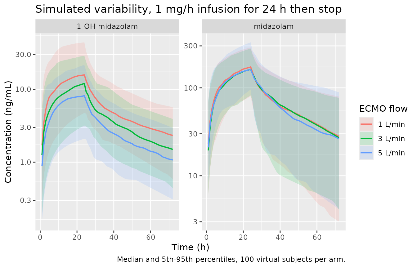
The flow arms separate for 1-OH-midazolam and are superimposed for midazolam, which is the structural signature of a covariate acting on the metabolite’s clearance alone.
On-ECMO versus post-ECMO
The two models were fit independently, so a direct comparison of their typical profiles is the natural summary of the paper’s clinical message. The post-ECMO model has a much smaller central volume (8.25 L vs 36.7 L) and a faster formation clearance (5.44 L/h vs 3.26 L/h).
ev_cmp <- make_arm(flow = 2.7, n = 1L, amt = 24, rate = 1,
                   times = seq(0, 72, by = 0.5))

sim_phase <- dplyr::bind_rows(
  rxode2::rxSolve(rxode2::zeroRe(ui_ecmo), events = ev_cmp,
                  useLinCmt = FALSE, returnType = "data.frame") |>
    dplyr::mutate(phase = "on ECMO (flow 2.7 L/min)"),
  rxode2::rxSolve(rxode2::zeroRe(ui_post), events = ev_cmp,
                  useLinCmt = FALSE, returnType = "data.frame") |>
    dplyr::mutate(phase = "after ECMO")
)
#> ℹ omega/sigma items treated as zero: 'etalcl_1ohm', 'etalcl_form_1ohm', 'etalvc', 'etalvp', 'etalvc_1ohm'
#> ℹ omega/sigma items treated as zero: 'etalcl_1ohm', 'etalcl_form_1ohm', 'etalvp', 'etalvc_1ohm'

sim_phase |>
  dplyr::filter(time > 0) |>
  tidyr::pivot_longer(c(Cc, Cc_1ohm), names_to = "analyte", values_to = "conc") |>
  dplyr::mutate(analyte = ifelse(analyte == "Cc", "midazolam", "1-OH-midazolam")) |>
  ggplot(aes(time, conc, colour = phase)) +
  geom_line(linewidth = 0.8) +
  facet_wrap(~analyte, scales = "free_y") +
  scale_y_log10() +
  labs(x = "Time (h)", y = "Concentration (ng/mL)", colour = NULL,
       title = "Typical profiles, 1 mg/h midazolam for 24 h then stop",
       caption = "modellib('Kim_2026_midazolam_ecmo') vs modellib('Kim_2026_midazolam_postecmo').")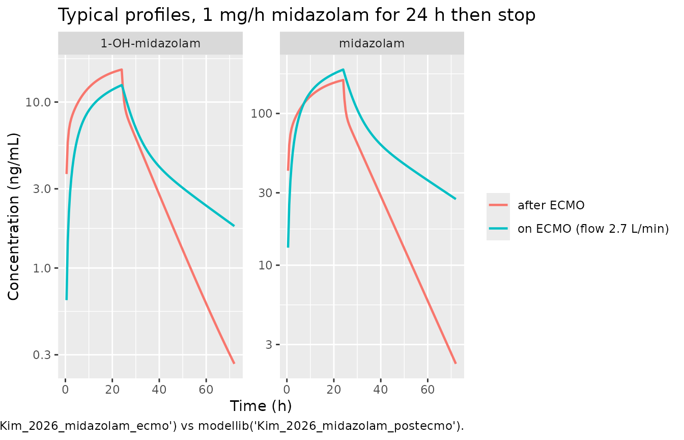
Assumptions and deviations
Errata and reporting gaps in the source
The covariate functional form is never stated. Supplementary Methods says continuous covariates were “centered on median values and evaluated using exponential, power, and proportional models” but never says which form was retained for ECMO flow rate. The median-normalized proportional form was recovered by fitting the paper’s own Figure 1A. Of the candidates, only it fits: RMSE 0.011 against the five published labels, versus 0.094 for the power form; the plain proportional form
1 + theta * (F - Fm)would require a negative median of -2.3 L/min, and the exponential form overshoots grossly (predicting 1.40 at 2 L/min against a published 1.16). Two independent corroborations: the main text describes the relationship as a “linear rise”, which excludes the power and exponential forms, and the Methods’ own wording specifies median centering.The centering median is published nowhere. Supplementary Table S1 tabulates every other screened covariate – age, weight, sex, indication, AST, ALT, serum creatinine, ECMO duration – but omits ECMO flow rate. The value 2.7 L/min is figure-derived, not paper-reported: solving for the median at each of the four non-trivial Figure 1A points gives 2.66, 2.47, 2.72, and 2.71 L/min. This is flagged inline in the model file’s
ini()comment and incovariateData[[Q_ECMO]]$notes. It is a plausible adult VA-ECMO flow, and the Figure 1A replication above confirms it end-to-end through the ODE system, but a reader who obtains the control stream should verify it.Figure 1B is not reproducible from Table 1. See the dedicated section above. The published 70%-decrement gradient (20.62 h down to 15.90 h) cannot be generated by any covariate form acting on
CL_1-OH, because the metabolite is formation-rate-limited and its decline tracks the flow-independent parent. The published across-flow mean (18.03 h) does match the simulated value (18.12 h). The model reproduces Table 1 faithfully; the inconsistency is in the source.The paper contradicts itself about which analyte Figures 1A and 1B show. The Figure 1B caption, the Supplementary Fig. S6 caption, and the Supplementary Methods all say “midazolam”; the main text Results paragraph says “1-hydroxymidazolam”. It must be the metabolite – the covariate acts only on
CL_1-OH, so a midazolam-based version of either figure would be flat across flow. The Figure 1A table above demonstrates exactly this: simulated midazolam concentration at 24 h is identical at all five flows. Supplementary Fig. S8, which plots 1-OH profiles with the 70% points marked, corroborates the metabolite reading.An ETA correlation is reported for an eta that has no reported variance. Table 1 has a row under “ETA correlation” labelled
omega^2 CL1-OH MDZ, omega^2 Q1-OH MDZwith a value of 0.228 (bootstrap 95% CI 0-0.56, on-ECMO model only). The Random effects block above it reports variances for five etas, and none of them is an eta onQ_1-OH MDZ. The correlation therefore names an eta whose variance is published nowhere and cannot be built without inventing one, so it is not encoded. Note also that if the row were instead a covariance between the two 1-OH etas that do exist, 0.228 would imply a correlation of0.228 / sqrt(0.246 * 0.137)= 1.24, which is impossible – so under any reading the number is a correlation coefficient rather than a covariance. Its bootstrap CI includes zero. The row is recorded here verbatim so a reader holding the control stream can restore it.Supplementary Fig. S7’s y-axis units appear to be wrong by a factor of 1000. The axis reads “AUC0-48 of 1-OH MDZ (ngh/mL)” but the plotted values (roughly 0.4-0.7 at a 1 mg/h infusion) are consistent with mgh/L, i.e. ug*h/mL. Only the trend direction from that figure is used here.
Supplementary Table S2 tabulates a noisy, non-monotonic “time to target concentration” (13-21 h) across the 50 dose-by-flow scenarios, which is not consistent with the smooth monotonic curve of Figure 1B. Those values come from Monte Carlo simulation with between-subject variability (500 replicates of 50 scenarios per Supplementary Methods), so they are not directly comparable to a typical-value reproduction and are not used as a validation target.
Encoding decisions
Parent-to-metabolite transfer is 1:1 in midazolam-equivalent mass. The paper states no molar conversion factor and reports no fraction metabolised, and
CL_MFis the only parent elimination pathway, so all parent mass is transferred. This matches the convention used bymodellib("Franken_2017_midazolam"). A true molar correction (MW 341.8 / 325.8 = 1.049) would rescaleCL_1-OHand the 1-OH volumes by under 5%, and cannot be applied without knowing whether the assay already reported midazolam equivalents.Random effects are read as variances, not standard deviations. Justified in the Source trace section above: the printed parenthetical is
100 * sqrt(omega^2)for all nine entries. Independently, the residual RSEs are consistent with a variance scale – the RSE of an estimated variance is roughlysqrt(2/N), and the parent’s 13.3% implies about 113 observations, plausible for 19 serially sampled patients, whereas an SD scale would imply about 28.The post-ECMO
omega^2 Vc,MDZ = 0 FIXis omitted rather than written asfixed(0). A zero-variance diagonal makes OMEGA singular and breaks the Cholesky sampler thatrxSolve()uses, and a zero-variance eta contributes nothing, so the two encodings are mathematically identical. Same handling asmodellib("Wattanakul_2024_primaquine_motherinfant").Concentrations are reported in ng/mL, matching the assay described in Supplementary Methods (LLOQ 25 ng/mL midazolam, 5 ng/mL 1-OH-midazolam). The ODE states hold mg and the volumes are litres, so
model()scales amount/volume by 1000.Evaluated-but-not-retained covariates are recorded in each model’s
covariatesDataExcludedmetadata rather thancovariateData, because the paper reports no effect estimate for any of them. Nine come from the screened-covariate list in Supplementary Methods, “Covariate model development” (age, weight, albumin, AST, ALT, serum creatinine, sex, concomitant sufentanil, concomitant remifentanil).ECMO_PUMP_SPEEDis listed alongside them with a narrower claim: the supplement documents pump speed as collected (“Clinical data collection” and “ECMO system”) but does not name it among the screened covariates, and it does not appear in Table 1. It is worth singling out because Kim 2026 recorded both pump speed and flow rate and retained only flow rate, the exact reverse ofmodellib("Yang_2017_remifentanil"), which tested both and retained only pump speed.checkModelConventions()emits one known false positive on this model. It flagse_q_ecmo_cl_1ohmas “a reversed-order covariate effect (e_<param>_<cov>)”. The name is in fact the canonicale_<cov>_<param>order, with covariateq_ecmoand parametercl_1ohm. The heuristic misfires because it splits on underscores and finds that the first token,q, is a bare PK parameter name (intercompartmental clearance) while a later token,ecmo, is a known covariate token – a collision that is unavoidable for any covariate whose canonical name begins withQ_. The parameter is deliberately not renamed, because any name that dodges the heuristic would no longer match the covariate’s canonical spelling. The check reports it as a warning, not an error, so it does not blockbuildModelDb().Q_ECMOis a new canonical covariate column, registered ininst/references/covariate-columns.mdalongside this extraction and named into theQ_circuit-flow family (withQ_CVVH,Q_TOTAL_LPM,QBL) rather than the device-prefixedECMO_family. It is the first time the library retains ECMO flow rate as a covariate in a final model.
Simulation assumptions
- No observed data are available, so every figure uses virtual cohorts.
- The paper does not report the observed distribution of ECMO flow rates, so the flow arms are the 1-5 L/min integer grid the paper itself simulates.
-
Q_ECMOis treated as constant per subject; it is naturally time-varying (flow is titrated during weaning) but the paper does not state the time resolution used in the fit. - Dosing is simulated as a clean 1 mg/h infusion or a single 5 mg bolus. Real patients received physician-titrated infusions with supplementary boluses.