Safinamide PK and ON-time (Loprete 2016)
Source:vignettes/articles/Loprete_2016_safinamide.Rmd
Loprete_2016_safinamide.RmdModel and source
Loprete 2016 reports two population models built from the safinamide phase 3 programme, and this vignette validates both. They are packaged as two model files because the authors fitted them to different datasets and the final PD model contains no exposure term, so they are independent rather than coupled (see “Why two model files” below).
- Citation: Loprete L, Leuratti C, Cattaneo C, Thapar MM, Farrell C, Sardina M. Population pharmacokinetic and pharmacodynamic analyses of safinamide in subjects with Parkinson’s disease. Pharmacol Res Perspect 2016;4(5):e00251. doi:10.1002/prp2.251.
- Article: https://doi.org/10.1002/prp2.251
- PubMed Central: https://www.ncbi.nlm.nih.gov/pmc/articles/PMC5045937/
| Model file | What it describes | Fitted to |
|---|---|---|
Loprete_2016_safinamide |
One-compartment oral popPK (model 110a) | 623 patients, 2719 concentrations, Studies 015 + 016 |
Loprete_2016_safinamide_ontime |
Linear ON-time disease-progression / treatment-effect model (model 915) | 668 patients, 3603 ON-time observations, Study 016 only |
| Model | Description |
|---|---|
| Loprete_2016_safinamide | One-compartment population pharmacokinetic model with first-order absorption and first-order elimination for oral safinamide in patients with Parkinson’s disease on stable dopamine-agonist or levodopa therapy, pooled from two phase 3 randomized placebo-controlled trials (Study 015 and Study 016; Loprete 2016 model 110a). Apparent oral clearance and apparent volume of distribution are allometrically scaled on body weight about a 70 kg reference with structural exponents of 0.75 and 1. Safinamide exposure was about 30% lower in Study 016 (tablets of safinamide free base) than in Study 015 (gelatin capsules of safinamide methanesulfonate); the authors carried that difference as a relative bioavailability factor of 0.724 on the depot rather than as separate clearance and volume estimates, switched on by the binary STUDY_016 indicator, so the default ini() values are the Study 015 reference parameters. Interindividual variability is estimated on CL/F and Vd/F; the authors set the IIV on KA and the additive residual error term to zero in the final model because both were poorly estimated. Residual error is proportional. Age, sex, creatinine clearance, race and levodopa exposure were screened and not retained. |
| Loprete_2016_safinamide_ontime | Linear disease-progression and treatment-effect model for daily ON-time (ON-time plus ON-time with minor dyskinesia, recorded in the Hauser patient diary over an 18 h window) in patients with Parkinson’s disease and motor fluctuations on stable levodopa, from the safinamide phase 3 Study 016 (Loprete 2016 model 915). ON-time is the individual observed baseline plus an intercept offset plus a slope times study time in 4-week months: ontime = ONTIME_BL + (intplac + inttreat * ON_TREATMENT) + slopplac * time. The placebo intercept offset was small, poorly estimated and set to zero; the safinamide effect on the slope was also set to zero, so safinamide acts purely as an instantaneous 0.728 h upward shift attained by the first post-baseline visit at week 4, after which ON-time rises with the same slope as placebo. Interindividual variability is additive on the intercept and on the slope; the baseline carries no random effect because individual observed baselines are supplied as data. Residual error is additive. This model has NO drug PK input: safinamide average 24 h concentration, safinamide dose, age and levodopa exposure were all screened as covariates and none improved the fit, so the drug effect is carried entirely by a treatment-arm indicator. It is therefore a companion to, but not coupled with, the population PK model in the same paper (modellib(‘Loprete_2016_safinamide’)). |
Why two model files
The paper’s title promises a PKPD analysis, and the Methods do set
out to test safinamide exposure on the ON-time response. That test
failed. Loprete 2016 computed a per-visit average safinamide
concentration (SAAV) from each patient’s individual
clearance in the population PK run, screened it on both the intercept
and the slope of the ON-time trajectory, and retained neither: the
confidence intervals of the exposure effect included the null, and
Figure 5 shows no exposure-response trend. The categorical safinamide
dose was screened too, with the same outcome.
The published final PD model (model 915) therefore has no PK input at all. Its drug effect is a binary treatment-arm switch. Encoding it as a PK-coupled model would misrepresent what the authors fitted, so the two models are separate files and this vignette validates each on its own terms. The standing policy is to build the models as the authors built them.
Population
Population PK (both studies). 623 patients contributing 2719 safinamide concentration records: 177 patients / 1099 concentrations from Study 015 (Stocchi 2012; early idiopathic Parkinson’s disease on a stable dose of a single dopamine agonist, receiving gelatin capsules of safinamide methanesulfonate titrated to 100 or 200 mg/day) and 446 patients / 1620 concentrations from Study 016 (Borgohain 2014; Parkinson’s disease with motor fluctuations on stable levodopa, receiving tablets of safinamide free base at 50 or 100 mg/day). Both trials ran 24 weeks and both excluded placebo-arm records from the PK dataset. Loprete 2016 Table 1: median age 60.0 years (range 31.0-82.0), median baseline body weight 64.0 kg (range 33.5-102), median baseline creatinine clearance 75.5 mL/min (range 25.3-201), 431 male (69%) / 192 female (31%). Race was recorded only in Study 016 (80.3% Asian, 19.5% White), so 28.4% of the pooled cohort has race not available. Renal function spanned normal to moderate impairment: 259 (42%) normal, 307 (49%) mild (50-80 mL/min), 57 (9%) moderate (< 50 mL/min), and no patient had severe impairment (< 10 mL/min). Bioanalysis was by validated LC-MS/MS with a lower limit of quantification of 20 ng/mL; below-limit records were excluded rather than imputed.
ON-time model (Study 016 only). 668 patients contributing 3603 ON-time observations at weeks 1 (baseline), 4, 8, 12, 18 and 24. Loprete 2016 Table 2: median age 60.0 years (range 34.0-80.0), median baseline body weight 62.0 kg (range 33.5-120), median baseline creatinine clearance 73.5 mL/min (range 25.8-199), 480 male (71.9%) / 188 female (28.1%), 538 Asian (80.5%) / 129 White (19.3%) / 1 Other. Each observation is the average, over the 2 to 5 diary recording days preceding the visit, of ON-time plus ON-time with minor dyskinesia during the 18 h window 0600-2400 of the Hauser patient diary. Levodopa dosing was largely stable through the trial: 11/668 (2%) of patients increased their dose and 51/668 (8%) decreased it.
The same information is available programmatically from each model’s
population metadata, e.g.
rxode2::rxode(readModelDb("Loprete_2016_safinamide"))$population.
Source trace
Every ini() entry in both model files carries an in-file
comment naming its source location. The table below collects them for
review.
| Model | Equation / parameter | Value | Source location |
|---|---|---|---|
| PK | lka |
0.582 /h | Table 3, row KA (h-1) (%RSE 21.6; 95% CI
0.335-0.829) |
| PK | lcl |
3.59 L/h | Table 3, row CL/F (L/h) (%RSE 2.67; 95% CI 3.40-3.78);
Table 3 footnote fixes the reference at 70 kg |
| PK | lvc |
120 L | Table 3, row Vd/F (L) (%RSE 4.38; 95% CI 110-130) |
| PK | lfdepot |
1 (anchor) | Methods, Structural model: “Frel was set to 1 for the Study 015” |
| PK | e_study_016_fdepot |
log(0.724) | Table 3, row F (STUD016) (%RSE 2.49; 95% CI
0.689-0.759) |
| PK | e_wt_cl |
0.75 | Results, PK analysis and final model: scaling factor
(WGT/70)^0.75 on CL/F |
| PK | e_wt_vc |
1 | Results: scaling factor (WGT/70) on Vd/F; Discussion
restates it as “linearly for Vd/F” |
| PK | etalcl |
0.0772 | Table 3, row x2 CL (%RSE 11.2; CV 27.8%) |
| PK | etalvc |
0.0892 | Table 3, row x2 Vd (%RSE 17.2; CV 29.9%) |
| PK | etalka |
0 | Results, model 110a: IIV on KA set to zero (%RSE 71, shrinkage 60%) |
| PK | propSd |
sqrt(0.0885) | Table 3, row r2 prop (%RSE 5.11; CV 29.7%) |
| PK | addSd |
0 | Results, model 110a: additive residual error set to zero (%RSE 102) |
| PK | covariate power form | n/a | Equation 1: TVPi = theta1 * (COVi / COVST)^theta2
|
| PK | binary covariate form | n/a | Equation 2: TVPi = theta1 * theta2^INDi
|
| PK | IIV form | n/a | Equation 3: Pi = TVP * exp(eta_Pi) (log-normal) |
| PK | residual error form | n/a | Equation 4: combined proportional plus additive |
| PD | intplac |
0 | Table 4, row Intercept (INT PLAC) (h): 0 FIX |
| PD | inttreat |
0.728 h | Table 4, row INT TREAT (h) (%RSE 15.0; 95% CI
0.514-0.942) |
| PD | slopplac |
0.117 h/month | Table 4, row Slope (SLOP PLAC) (h/month) (%RSE 17.0;
95% CI 0.0780-0.156) |
| PD | etaintercept |
3.29 | Table 4, row x2 INT PLAC (h) (%RSE 7.93; SD 1.81) |
| PD | etaslope |
0.130 | Table 4, row x2 SLOP PLAC (h/month) (%RSE 10.5; SD
0.361) |
| PD | addSd |
sqrt(1.19) | Table 4, row Residual variability r2 add (%RSE 5.59; SD
1.09 h) |
| PD | structural equation | n/a | Equation 7 reduced by INTPLAC = 0 and
SLOPTREAT = 0; restated in the Table 4 caption as
PD = BL + INTPLAC + INTTREAT + SLOPPLAC * TIMEmonths
|
| PD | IIV form | n/a | Equation 8: Pi = TVP + eta_Pi (additive) |
| PD | residual error form | n/a | Equation 9: additive only |
The Table 3 and Table 4 variance columns are read as
variances, not standard deviations, and the paper’s own
printed summary columns settle that reading:
sqrt(0.0772) = 0.278 matches the printed CV of 27.8%,
sqrt(0.0892) = 0.299 matches 29.9%,
sqrt(0.0885) = 0.297 matches 29.7%,
sqrt(3.29) = 1.81 matches the printed SD of 1.81,
sqrt(0.130) = 0.361 matches 0.361, and
sqrt(1.19) = 1.09 matches 1.09 h.
# The printed CV / SD columns are what fix the variance-vs-SD reading of the
# 'x2' and 'r2' columns. If a future edit swapped a variance for an SD, this
# goes red. Deterministic arithmetic on the transcribed values -- no simulation.
stopifnot(
  abs(sqrt(0.0772) - 0.278) < 0.001, # Table 3 x2 CL  -> CV 27.8%
  abs(sqrt(0.0892) - 0.299) < 0.001, # Table 3 x2 Vd  -> CV 29.9%
  abs(sqrt(0.0885) - 0.297) < 0.001, # Table 3 r2 prop -> CV 29.7%
  abs(sqrt(3.29) - 1.81) < 0.005, # Table 4 x2 INT  -> SD 1.81 h
  abs(sqrt(0.130) - 0.361) < 0.005, # Table 4 x2 SLOP -> SD 0.361 h/month
  abs(sqrt(1.19) - 1.09) < 0.005 # Table 4 r2 add  -> SD 1.09 h
)
Part 1 – population pharmacokinetics
Typical-value covariate round trip
Loprete 2016 quotes four typical-value anchors that between them pin the allometric exponents, the reference weight and the relative bioavailability:
- Results: “CL/F and Vd/F estimates for the lightest (33 kg) and the heaviest patient (105 kg) were 2.04 and 4.87 L/h and 57 and 180 L, respectively.”
- Abstract and Discussion: for Study 016, “CL/F and Vd/F (95% CI) were 4.96 (4.73-5.21) L/h and 166 (158-174) L”.
The first set exercises the weight model, the second the
bioavailability model. Both are reproduced here by solving the packaged
model with the random effects zeroed and reading the individual
parameters back out of the solve, so the whole covariate path in
model() is exercised rather than the ini()
arithmetic alone.
mod_pk <- readModelDb("Loprete_2016_safinamide")
mod_pk0 <- rxode2::zeroRe(mod_pk)

obs_grid <- seq(0.25, 240, by = 0.25)

make_pk_typical <- function(id, wt, study016, dose = 100) {
  data.frame(
    id = id,
    time = c(0, obs_grid),
    evid = c(1L, rep(0L, length(obs_grid))),
    amt = c(dose, rep(NA_real_, length(obs_grid))),
    # Observation rows sit on the ODE state `central`, never on the algebraic
    # observable `Cc`; rxode2 returns Cc as a column at those rows anyway.
    cmt = c("depot", rep("central", length(obs_grid))),
    WT = wt,
    STUDY_016 = study016,
    study = ifelse(study016 == 1, "Study 016", "Study 015"),
    wt_label = paste0(wt, " kg")
  )
}

ev_typ <- dplyr::bind_rows(
  make_pk_typical(1L, 33, 0L), make_pk_typical(2L, 70, 0L),
  make_pk_typical(3L, 105, 0L), make_pk_typical(4L, 33, 1L),
  make_pk_typical(5L, 70, 1L), make_pk_typical(6L, 105, 1L)
)
stopifnot(!anyDuplicated(unique(ev_typ[, c("id", "time", "evid")])))

sim_typ <- rxode2::rxSolve(
  mod_pk0,
  events = ev_typ, returnType = "data.frame",
  keep = c("WT", "STUDY_016", "study", "wt_label")
)
#> ℹ omega/sigma items treated as zero: 'etalcl', 'etalvc', 'etalka'
#> Warning: multi-subject simulation without without 'omega'

par_typ <- sim_typ |>
  dplyr::distinct(id, study, WT, cl, vc) |>
  dplyr::arrange(study, WT)

par_typ |>
  dplyr::filter(study == "Study 015") |>
  dplyr::mutate(cl = round(cl, 3), vc = round(vc, 1)) |>
  dplyr::select(-id, -study) |>
  dplyr::rename(
    "Body weight (kg)" = WT,
    "CL/F (L/h)" = cl,
    "Vd/F (L)" = vc
  ) |>
  knitr::kable(
    caption = paste(
      "Study 015 typical values by body weight.",
      "Loprete 2016 Results publishes 2.04 / 3.59 / 4.87 L/h and",
      "57 / 120 / 180 L for 33 / 70 / 105 kg."
    )
)| Body weight (kg) | CL/F (L/h) | Vd/F (L) |
|---|---|---|
| 33 | 2.042 | 56.6 |
| 70 | 3.590 | 120.0 |
| 105 | 4.866 | 180.0 |
s015 <- par_typ |> dplyr::filter(study == "Study 015") |> dplyr::arrange(WT)

# Deterministic (random effects zeroed) closed-form quantities, so the bound is
# set by the precision the paper printed at rather than by any cohort spread.
# Clearances are published to three significant figures and volumes to whole
# litres, so half of the last printed digit is the right tolerance in each case:
# the model gives 56.571 L at 33 kg, which the paper prints as 57. A tolerance
# expressed as a PERCENTAGE would have to admit 0.9% to pass that row, which is
# looser than 3-significant-figure clearances deserve.
#
# This is the gate that catches a mis-typed allometric exponent (0.75 vs 1 moves
# the 33 kg clearance by 27%), a wrong reference weight, or a transposed CL/Vd
# pair.
stopifnot(
  max(abs(s015$cl - c(2.04, 3.59, 4.87))) < 0.005, # half of the last digit
  max(abs(s015$vc - c(57, 120, 180))) < 0.5 # published as whole litres
)
Apparent clearance and volume via PKNCA
The relative bioavailability model is validated the other way round:
rather than reading cl out of the solve (which returns the
Study 015 value regardless of arm, because STUDY_016 acts
on f(depot) and not on clearance), we integrate the
simulated profile and recover the apparent CL/F and
Vd/F that an external analyst would compute as dose over exposure. That
is the quantity Loprete 2016 quotes for Study 016, and recovering it
exercises the bioavailability term, the ODE, and the
central / vc * 1000 unit scaling in one pass.
nca_typ <- sim_typ |>
  # Only `!is.na(Cc)`: adding `time > 0` or `Cc > 0` would drop the time-zero
  # row that PKNCA needs to anchor AUC from 0.
  dplyr::filter(!is.na(Cc)) |>
  dplyr::select(id, time, Cc, study, wt_label)

nca_typ <- dplyr::bind_rows(
  nca_typ,
  nca_typ |>
    dplyr::distinct(id, study, wt_label) |>
    dplyr::mutate(time = 0, Cc = 0)
) |>
  dplyr::distinct(id, study, wt_label, time, .keep_all = TRUE) |>
  dplyr::arrange(id, time)

conc_typ <- PKNCA::PKNCAconc(
  nca_typ, Cc ~ time | study + wt_label + id,
  concu = "ng/mL", timeu = "h"
)
dose_typ <- PKNCA::PKNCAdose(
  ev_typ |>
    dplyr::filter(evid == 1L) |>
    dplyr::select(id, time, amt, study, wt_label),
  amt ~ time | study + wt_label + id,
  doseu = "mg"
)

intervals_typ <- data.frame(
  start = 0, end = Inf,
  cmax = TRUE, tmax = TRUE, aucinf.obs = TRUE,
  half.life = TRUE, cl.obs = TRUE, vz.obs = TRUE
)

res_typ <- PKNCA::pk.nca(
  PKNCA::PKNCAdata(conc_typ, dose_typ, intervals = intervals_typ)
)

# PKNCA returns cl.obs and vz.obs in dose / conc units, i.e. mg / (ng*h/mL) and
# mg / (ng/mL). Both are litre-scaled by 1000: 100 mg / 27830 ng*h/mL = 0.00359,
# and 0.00359 * 1000 = 3.59 L/h.
nca_typ_tbl <- as.data.frame(res_typ$result) |>
  dplyr::mutate(
    PPORRES = ifelse(PPTESTCD %in% c("cl.obs", "vz.obs"), PPORRES * 1000, PPORRES)
  )
# Reference side: the paper's own published typical values for a 70 kg patient.
# Study 015 is Table 3; Study 016 is the abstract / Discussion. The half-life
# is not tabulated by Loprete 2016 -- it is the closed form implied by the
# Table 3 estimates, log(2) * Vd/F / (CL/F) = log(2) * 120 / 3.59, which is
# identical in both arms because relative bioavailability cancels out of it.
thalf_closed_form <- log(2) * 120 / 3.59

published_pk <- tibble::tribble(
  ~study, ~cl.obs, ~vz.obs, ~half.life,
  "Study 015", 3.59, 120, thalf_closed_form,
  "Study 016", 4.96, 166, thalf_closed_form
)

cmp_pk <- nlmixr2lib::ncaComparisonTable(
  simulated = nca_typ_tbl |> dplyr::filter(wt_label == "70 kg"),
  reference = published_pk,
  by = "study",
  units = c(cl.obs = "L/h", vz.obs = "L", half.life = "h"),
  tolerance_pct = 20
)

knitr::kable(
  cmp_pk,
  caption = paste(
    "Apparent CL/F, Vz/F and terminal half-life recovered by PKNCA from the",
    "packaged model at 70 kg, against the values Loprete 2016 publishes.",
    "* marks a difference above 20%."
  ),
  align = c("l", "l", "r", "r", "r")
)| NCA parameter | study | Reference | Simulated | % diff |
|---|---|---|---|---|
| t½ (h) | Study 015 | 23.2 | 23.2 | +0.0% |
| t½ (h) | Study 016 | 23.2 | 23.2 | +0.0% |
| CL/F (L/h) | Study 015 | 3.59 | 3.59 | +0.0% |
| CL/F (L/h) | Study 016 | 4.96 | 4.96 | -0.0% |
| Vz/F (L) | Study 015 | 120 | 120 | +0.0% |
| Vz/F (L) | Study 016 | 166 | 166 | -0.1% |
get_typ <- function(study, code) {
  v <- nca_typ_tbl$PPORRES[
    nca_typ_tbl$study == study &
      nca_typ_tbl$wt_label == "70 kg" &
      nca_typ_tbl$PPTESTCD == code
  ]
  # A lookup that matches nothing returns numeric(0), and every downstream
  # all() would then pass vacuously. Fail loudly instead.
  if (length(v) != 1L) {
    stop("no unique ", code, " for ", study)
  }
  v
}

clf_015 <- get_typ("Study 015", "cl.obs")
clf_016 <- get_typ("Study 016", "cl.obs")
vzf_015 <- get_typ("Study 015", "vz.obs")
vzf_016 <- get_typ("Study 016", "vz.obs")
thalf_015 <- get_typ("Study 015", "half.life")

# Deterministic again (random effects zeroed), so these are numerical-accuracy
# bounds, not cohort bounds: the only error sources are the solver and the
# trapezoidal integration of a 0.25 h grid. 1% leaves ample room for those and
# still goes red on a mis-applied bioavailability (which would move CL/F by 38%)
# or a missing 1000x unit scale (which would move it by three orders).
stopifnot(
  abs(clf_015 - 3.59) / 3.59 < 0.01,
  abs(clf_016 - 4.96) / 4.96 < 0.01,
  abs(vzf_015 - 120) / 120 < 0.01,
  abs(vzf_016 - 166) / 166 < 0.01,
  abs(thalf_015 - thalf_closed_form) / thalf_closed_form < 0.01
)

# The relative bioavailability itself, recovered as the ratio of apparent
# clearances. Table 3 publishes F(STUD016) = 0.724.
stopifnot(abs(clf_015 / clf_016 - 0.724) < 0.005)
The model reproduces every published typical value. The recovered terminal half-life is 23.2 h, against the “approximately 22 h” that Loprete 2016’s Discussion quotes for safinamide. That 22 h is a literature value carried in from Marzo 2004 and Leuratti 2013 rather than an output of this analysis, so it is reported here for context and is deliberately not gated: the gate above is against the half-life the Table 3 parameters themselves imply.
Steady-state cohort and the per-subject dose / exposure identity
Safinamide was dosed once daily for 24 weeks in both trials, and the analysis dataset replaced runs of identical dose records with a steady-state record at a 24 h interval. The cohort below gives each arm the same body-weight distribution so that the only difference between the arms is relative bioavailability, which is what makes the arm contrast interpretable.
rxode2::rxSetSeed(20160711) # the paper's acceptance date

n_per_arm <- 200L
tau <- 24
n_days <- 14 # ~14 elimination half-lives; steady state is reached by ~day 5
t_last_dose <- (n_days - 1) * tau

# Body weight: log-normal matched to the Loprete 2016 Table 1 pooled median of
# 64 kg, with the spread chosen so the 2.5th / 97.5th percentiles sit inside the
# reported 33.5-102 kg range. Truncated to the reported range.
wt_draw <- function(n) {
  w <- stats::rlnorm(n, meanlog = log(64), sdlog = 0.20)
  pmin(pmax(w, 33.5), 102)
}

set.seed(20160711) # seeds the weight draw only; rxode2's RNG is set above
wt_common <- wt_draw(n_per_arm)

make_ss_arm <- function(study016, label, id_offset) {
  dose_rows <- tidyr::expand_grid(
    i = seq_len(n_per_arm),
    time = seq(0, t_last_dose, by = tau)
  ) |>
    dplyr::mutate(evid = 1L, amt = 100, cmt = "depot")
  # Observations only over the final dosing interval: that is the only window
  # the NCA and the profile figure use, and keeping the grid off the dose times
  # avoids an observation record sharing a timestamp with a dose record.
  obs_rows <- tidyr::expand_grid(
    i = seq_len(n_per_arm),
    time = seq(t_last_dose, t_last_dose + tau, by = 0.25)
  ) |>
    dplyr::mutate(evid = 0L, amt = NA_real_, cmt = "central")

  dplyr::bind_rows(dose_rows, obs_rows) |>
    dplyr::mutate(
      id = id_offset + i,
      WT = wt_common[i],
      STUDY_016 = study016,
      study = label
    ) |>
    dplyr::select(id, time, evid, amt, cmt, WT, STUDY_016, study) |>
    dplyr::arrange(id, time, dplyr::desc(evid))
}

ev_ss <- dplyr::bind_rows(
  make_ss_arm(0L, "Study 015", 0L),
  make_ss_arm(1L, "Study 016", 1000L)
)
# Disjoint IDs across arms: duplicate IDs are silently merged by rxSolve into a
# single subject receiving the summed dose.
stopifnot(!anyDuplicated(unique(ev_ss[, c("id", "time", "evid")])))

sim_ss <- rxode2::rxSolve(
  mod_pk,
  events = ev_ss, returnType = "data.frame",
  keep = c("WT", "STUDY_016", "study")
)
#> ℹ omega/sigma items treated as zero: 'etalka'
At steady state, the area under the concentration-time curve over one
dosing interval satisfies AUCtau = F * Dose / CL exactly,
for every subject. That identity is the single most informative gate
available here: a wrong bioavailability, a wrong unit scale, a dropped
allometric term or a mis-declared dose all break it, and unlike a ratio
it cannot pass by dividing two equally wrong numbers.
ss_window <- sim_ss |>
  dplyr::filter(time >= t_last_dose, !is.na(Cc)) |>
  dplyr::select(id, time, Cc, study, WT, cl)

conc_ss <- PKNCA::PKNCAconc(
  ss_window |> dplyr::select(id, time, Cc, study),
  Cc ~ time | study + id,
  concu = "ng/mL", timeu = "h"
)
dose_ss <- PKNCA::PKNCAdose(
  ev_ss |>
    dplyr::filter(evid == 1L, time == t_last_dose) |>
    dplyr::select(id, time, amt, study),
  amt ~ time | study + id,
  doseu = "mg"
)

intervals_ss <- data.frame(
  start = t_last_dose, end = t_last_dose + tau,
  cmax = TRUE, tmax = TRUE, cmin = TRUE, cav = TRUE, auclast = TRUE
)

res_ss <- PKNCA::pk.nca(
  PKNCA::PKNCAdata(conc_ss, dose_ss, intervals = intervals_ss)
)

auctau <- as.data.frame(res_ss$result) |>
  dplyr::filter(PPTESTCD == "auclast") |>
  dplyr::select(study, id, auctau = PPORRES)

per_subject <- ss_window |>
  dplyr::distinct(id, study, WT, cl) |>
  dplyr::left_join(auctau, by = c("id", "study")) |>
  dplyr::mutate(
    # F is 1 in Study 015 and 0.724 in Study 016 (Table 3).
    fdepot = ifelse(study == "Study 016", 0.724, 1),
    # AUCtau in ng*h/mL, dose 100 mg = 1e8 ng, so CL in mL/h; /1000 -> L/h.
    cl_from_auc = fdepot * 100 * 1e6 / auctau / 1000,
    pct_err = 100 * (cl_from_auc - cl) / cl
  )
stopifnot(nrow(per_subject) == 2L * n_per_arm, !anyNA(per_subject$auctau))
# Per-subject mass balance. The residual is numerical (trapezoidal integration
# of a 0.25 h grid over a broad peak, plus the small shortfall of a 14-day
# profile from exact steady state), not stochastic, so it is tight for every
# subject regardless of which cohort was drawn. Assert on the centre and on a
# robust quantile rather than on the extreme, per the repo's vignette policy.
stopifnot(
  abs(stats::median(per_subject$pct_err)) < 1,
  stats::quantile(abs(per_subject$pct_err), 0.9) < 2
)

# Arm contrast. Both arms share one body-weight vector, so the ratio of median
# exposures estimates the relative bioavailability directly. This one IS a
# cohort statistic, so the bound admits the sampling noise of a 200-subject
# median under ~28% CV on clearance (median SE about 2.5% per arm).
auc_ratio <- stats::median(per_subject$auctau[per_subject$study == "Study 016"]) /
  stats::median(per_subject$auctau[per_subject$study == "Study 015"])
stopifnot(abs(auc_ratio / 0.724 - 1) < 0.15)

# And the deterministic version of the same contrast, which has no sampling
# noise at all and pins the 30%-lower-exposure claim of the Discussion exactly.
stopifnot(abs(clf_015 / clf_016 - 0.724) < 0.005)
The simulated Study 016 to Study 015 exposure ratio is 0.756, against
the published relative bioavailability of 0.724. Loprete 2016’s
Discussion states the observed Study 016 concentrations were
“approximately 30% lower”, which is the same statement
(1 - 0.724 = 27.6%).
| Study | Parameter | Median | 5th pctile | 95th pctile |
|---|---|---|---|---|
| Study 015 | AUClast (ng*h/mL) | 28600.00 | 17400.00 | 46100.00 |
| Study 015 | Cavg (ng/mL) | 1190.00 | 725.00 | 1920.00 |
| Study 015 | Cmax (ng/mL) | 1530.00 | 968.00 | 2360.00 |
| Study 015 | Cmin (ng/mL) | 876.00 | 372.00 | 1520.00 |
| Study 015 | Tmax (h) | 4.25 | 3.75 | 4.25 |
| Study 016 | AUClast (ng*h/mL) | 21600.00 | 13800.00 | 35000.00 |
| Study 016 | Cavg (ng/mL) | 900.00 | 575.00 | 1460.00 |
| Study 016 | Cmax (ng/mL) | 1150.00 | 736.00 | 1710.00 |
| Study 016 | Cmin (ng/mL) | 629.00 | 317.00 | 1140.00 |
| Study 016 | Tmax (h) | 4.25 | 4.00 | 4.25 |
Replicating Figure 1
Loprete 2016 Figure 1 plots every observed safinamide concentration
against time after dose, on linear and logarithmic axes, and notes two
apparent peaks that the authors attribute to pooling samples drawn at
different study visits rather than to absorption. Study 015 sampled at 5
h after the first dose and then at any time up to 8 h post-dose at later
visits; Study 016 sampled at baseline, week 4, week 12 and week 24. The
panel below is the model’s analogue: simulated steady-state
concentrations including residual error (sim, which carries
the proportional residual error; Cc is the individual
prediction without it) over the first 8 h after a dose.
fig1_dat <- sim_ss |>
  dplyr::filter(
    time >= t_last_dose, time <= t_last_dose + 8, !is.na(sim)
  ) |>
  dplyr::mutate(tad = time - t_last_dose) |>
  dplyr::filter(sim > 0)

ggplot(fig1_dat, aes(tad, sim)) +
  geom_point(alpha = 0.06, size = 0.5) +
  stat_summary(
    fun = stats::median, geom = "line",
    colour = "#1b6ca8", linewidth = 0.9
  ) +
  facet_wrap(~study) +
  scale_y_log10() +
  labs(
    x = "Time after dose (h)",
    y = "Safinamide plasma concentration (ng/mL, log scale)",
    title = "Simulated steady-state concentrations after 100 mg once daily",
    caption = paste(
      "Analogue of Figure 1 of Loprete 2016 (observed concentrations vs time",
      "after dose). Blue line is the median. The Study 016 panel sits lower by",
      "the relative bioavailability factor of 0.724."
    )
  ) +
  theme_minimal()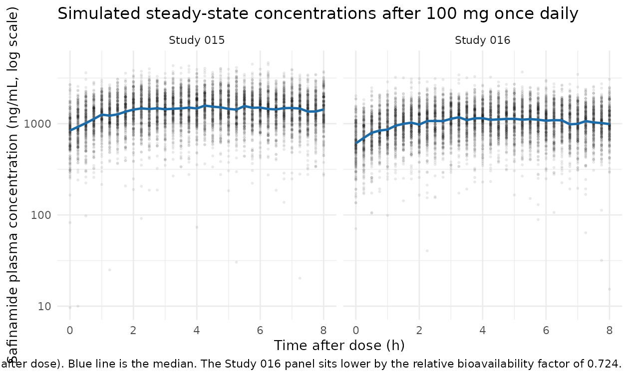
The horizontal grey band of the source figure below 20 ng/mL is absent here because the model emits continuous concentrations: Loprete 2016 excluded all below-quantification-limit records rather than imputing them, so no simulated counterpart of that censoring is applied.
Part 2 – ON-time disease progression and treatment effect
The final ON-time model is
ontime = ONTIME_BL + (intplac + inttreat * ON_TREATMENT) + slopplac * timewith intplac fixed at 0, inttreat = 0.728
h, slopplac = 0.117 h/month, and time measured in 4-week
months. There is no drug input and no ODE state.
The time unit
Loprete 2016’s dataset carries TIME in hours from the
baseline visit, while SLOPPLAC is reported per month. The
paper’s own arithmetic pins the month at four weeks: the Discussion
states that a slope of 0.117 h/month “would lead to an average increase
of 0.70 h over the duration of the study”, and
0.70 / 0.117 = 5.98, so the 24-week study is 6 months and
one month is 4 weeks = 672 h. The model file’s time unit is the month;
convert a dataset in hours by dividing by 672.
Typical-value trajectories (Figure 4)
Loprete 2016 Figure 4 plots observed ON-time and change from baseline against time by treatment arm, and the Discussion quotes two numeric anchors from it: the placebo arm gains an average of 0.70 h of ON-time over the study, and the safinamide arms gain 1.43 h, so that “at the end of the 6 months of study, ‘ON time’ duration after safinamide treatment was two times longer than after placebo administration”.
mod_pd <- readModelDb("Loprete_2016_safinamide_ontime")
mod_pd0 <- rxode2::zeroRe(mod_pd)

# Baseline ON-time is NOT reported by Loprete 2016. It is supplied here purely
# as an illustrative anchor -- 9.0 h, half the paper's 18 h (0600-2400) diary
# recording window -- and the invariance check below establishes that no
# quantitative claim in this section depends on the choice.
ontime_bl_illustrative <- 9.0

make_pd_arm <- function(id, on_treatment, bl, times = seq(0, 6, by = 0.05)) {
  data.frame(
    id = id,
    time = times,
    evid = 0L,
    amt = 0,
    ONTIME_BL = bl,
    ON_TREATMENT = on_treatment,
    arm = ifelse(on_treatment == 1L, "Safinamide", "Placebo")
  )
}

ev_pd_typ <- dplyr::bind_rows(
  make_pd_arm(1L, 0L, ontime_bl_illustrative),
  make_pd_arm(2L, 1L, ontime_bl_illustrative),
  # Two extra subjects at different baselines, used only by the invariance check.
  make_pd_arm(3L, 0L, 5.0),
  make_pd_arm(4L, 1L, 13.0)
)

sim_pd_typ <- rxode2::rxSolve(
  mod_pd0,
  events = ev_pd_typ, returnType = "data.frame",
  keep = c("ONTIME_BL", "ON_TREATMENT", "arm")
) |>
  dplyr::mutate(cfb = ontime - ONTIME_BL)
#> ℹ omega/sigma items treated as zero: 'etaintercept', 'etaslope'
#> Warning: multi-subject simulation without without 'omega'

ggplot(
  sim_pd_typ |> dplyr::filter(id %in% c(1, 2)),
  aes(time * 4, cfb, colour = arm)
) +
  geom_line(linewidth = 0.9) +
  geom_hline(yintercept = 0, linetype = "dotted", colour = "grey50") +
  scale_x_continuous(breaks = seq(0, 24, by = 4)) +
  labs(
    x = "Study time (weeks)",
    y = "Change from baseline in daily ON-time (h)",
    colour = "Arm",
    title = "Typical-value ON-time trajectories (model 915)",
    caption = paste(
      "Analogue of Figure 4 of Loprete 2016. The safinamide arm is offset by",
      "the 0.728 h instantaneous treatment effect and then rises with the",
      "same slope as placebo."
    )
  ) +
  theme_minimal()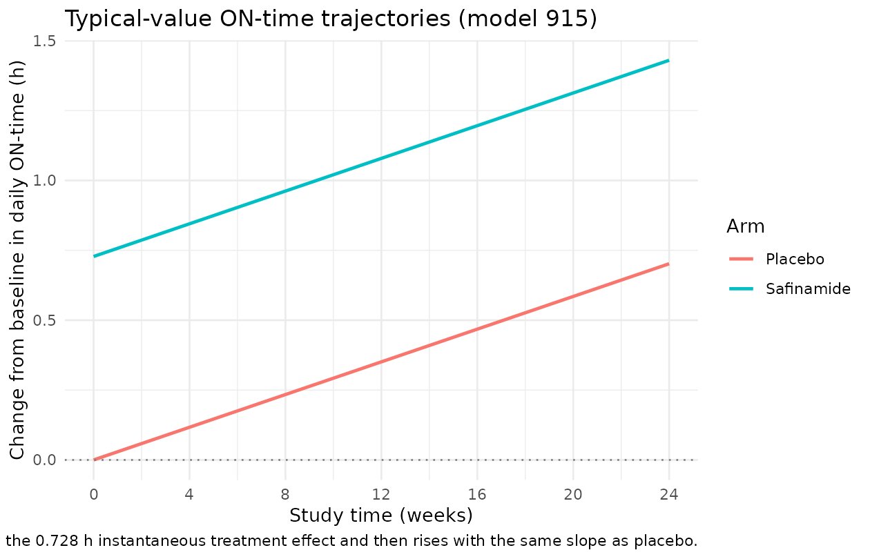
cfb_at_end <- function(subject_id) {
  v <- sim_pd_typ$cfb[sim_pd_typ$id == subject_id & abs(sim_pd_typ$time - 6) < 1e-9]
  if (length(v) != 1L) {
    stop("no unique end-of-study row for id ", subject_id)
  }
  v
}

cfb_placebo <- cfb_at_end(1)
cfb_safinamide <- cfb_at_end(2)

# Deterministic typical-value predictions, so these reproduce the published
# numbers to the precision they were printed at. 0.005 h is half of the last
# printed digit.
stopifnot(
  abs(cfb_placebo - 0.70) < 0.005, # Discussion: "an average increase of 0.70 h"
  abs(cfb_safinamide - 1.43) < 0.005 # Discussion: "estimated to be 1.43 h"
)

# "Two times longer" -- the ratio of the two INCREASES, not of the ON-time
# durations themselves. 1.43 / 0.702 = 2.04.
stopifnot(abs(cfb_safinamide / cfb_placebo - 2) < 0.15)

# The change from baseline is exactly invariant to ONTIME_BL, which is what
# licenses the illustrative baseline used above. Exact equality is correct here
# because the model is additive in ONTIME_BL -- this is not a cohort statistic.
stopifnot(
  abs(cfb_at_end(3) - cfb_placebo) < 1e-9,
  abs(cfb_at_end(4) - cfb_safinamide) < 1e-9
)| Arm | Published | Simulated |
|---|---|---|
| Placebo | 0.70 h | 0.702 h |
| Safinamide | 1.43 h | 1.430 h |
| Ratio (safinamide / placebo) | about 2 | 2.04 |
The instantaneous nature of the safinamide effect is the model’s
central claim: SLOPTREAT was estimated at essentially zero
and set to zero in model 908 without any change in objective function,
so the safinamide arms and the placebo arm share one slope and the
entire treatment effect is the intercept offset attained by the first
post-baseline visit at week 4.
Between-subject and residual variability
Loprete 2016 reports unusually large variability for this model: “interindividual CV for the estimated parameters (defined as SD/Estimate) ranging between 250% and 300%”, and a residual SD of 1.09 h.
# Reproduces the paper's own SD/Estimate definition from the Table 4 values.
cv_inttreat <- 100 * sqrt(3.29) / 0.728
cv_slopplac <- 100 * sqrt(0.130) / 0.117
stopifnot(
  cv_inttreat > 240, cv_inttreat < 260,
  cv_slopplac > 295, cv_slopplac < 320
)
The intercept CV is 249% and the slope CV is 308%, bracketing the paper’s stated 250-300% range (the slope sits marginally above it).
rxode2::rxSetSeed(20160711)

n_pd_arm <- 200L
make_pd_cohort <- function(n, on_treatment, id_offset, arm_label,
                           times = seq(0, 6, by = 0.25)) {
  tidyr::expand_grid(i = seq_len(n), time = times) |>
    dplyr::mutate(
      id = id_offset + i,
      evid = 0L,
      amt = 0,
      ONTIME_BL = ontime_bl_illustrative,
      ON_TREATMENT = on_treatment,
      arm = arm_label
    ) |>
    dplyr::select(id, time, evid, amt, ONTIME_BL, ON_TREATMENT, arm)
}

ev_pd_vpc <- dplyr::bind_rows(
  make_pd_cohort(n_pd_arm, 0L, 0L, "Placebo"),
  make_pd_cohort(n_pd_arm, 1L, 1000L, "Safinamide")
)
stopifnot(!anyDuplicated(unique(ev_pd_vpc[, c("id", "time", "evid")])))

sim_pd_vpc <- rxode2::rxSolve(
  mod_pd,
  events = ev_pd_vpc, returnType = "data.frame",
  keep = c("ONTIME_BL", "ON_TREATMENT", "arm")
) |>
  dplyr::mutate(cfb_obs = sim - ONTIME_BL)

sim_pd_vpc |>
  dplyr::group_by(arm, time) |>
  dplyr::summarise(
    Q05 = stats::quantile(cfb_obs, 0.05),
    Q50 = stats::quantile(cfb_obs, 0.50),
    Q95 = stats::quantile(cfb_obs, 0.95),
    .groups = "drop"
  ) |>
  ggplot(aes(time * 4, Q50, colour = arm, fill = arm)) +
  geom_ribbon(aes(ymin = Q05, ymax = Q95), alpha = 0.18, colour = NA) +
  geom_line(linewidth = 0.9) +
  geom_hline(yintercept = 0, linetype = "dotted", colour = "grey50") +
  scale_x_continuous(breaks = seq(0, 24, by = 4)) +
  labs(
    x = "Study time (weeks)",
    y = "Change from baseline in daily ON-time (h)",
    colour = "Arm", fill = "Arm",
    title = "Simulated ON-time response, 200 subjects per arm",
    caption = paste(
      "Median and 5th-95th percentile envelope, including additive residual",
      "error. Analogue of Figure 7A of Loprete 2016."
    )
  ) +
  theme_minimal()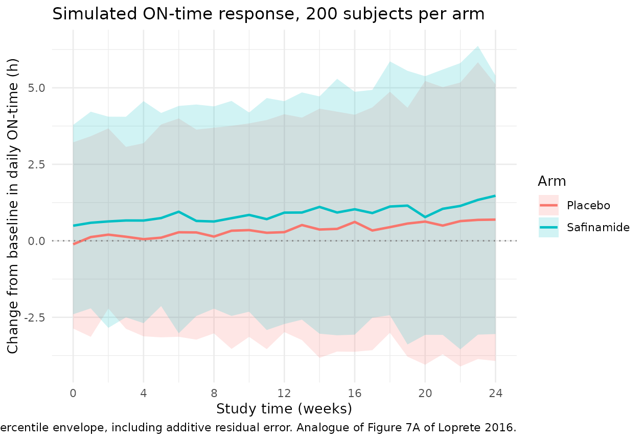
# The spread of the observed change from baseline at week 24 is a closed-form
# consequence of the Table 4 variances:
#   var = var(eta_intercept) + var(eta_slope) * t^2 + var(residual)
#       = 3.29 + 0.130 * 36 + 1.19
expected_sd_wk24 <- sqrt(3.29 + 0.130 * 6^2 + 1.19)

observed_sd_wk24 <- sim_pd_vpc |>
  dplyr::filter(abs(time - 6) < 1e-9) |>
  dplyr::pull(cfb_obs) |>
  stats::sd()

# A cohort statistic, so the bound admits sampling noise: the standard error of
# an SD from 400 draws is about SD/sqrt(2n), roughly 3.5% here. 25% leaves about
# seven standard errors of headroom and still goes red if a variance were read
# as a standard deviation (which would shrink the spread about two-fold) or if
# an eta were dropped.
stopifnot(abs(observed_sd_wk24 / expected_sd_wk24 - 1) < 0.25)

# The paper's qualitative claim that variability does not differ between arms
# (Results: "the variability of the ON-time did not differ between the treatment
# arms"). The model builds it in -- both arms share one eta structure -- so this
# checks the encoding, not the biology. Each arm is compared against the fixed
# closed-form expectation rather than against the other arm: racing two noisy
# standard deviations against each other is exactly the shape that passes where
# it is written and fails in CI. With 200 subjects per arm the standard error of
# an SD is about 5%, so 30% is roughly six standard errors of headroom; the two
# arms realised 3.11 and 2.75 h here, i.e. within 3% and 9% of expectation.
sd_by_arm <- sim_pd_vpc |>
  dplyr::filter(abs(time - 6) < 1e-9) |>
  dplyr::group_by(arm) |>
  dplyr::summarise(s = stats::sd(cfb_obs), .groups = "drop")
stopifnot(max(abs(sd_by_arm$s / expected_sd_wk24 - 1)) < 0.3)
The simulated week-24 standard deviation is 2.80 h against the closed-form 3.03 h implied by the Table 4 variances. The envelope is wide enough to span zero change in both arms, which is the quantitative form of the paper’s own caution that “the high variability in response and the limited duration of the study in relation to the persistence of the placebo effect reduce the possibility to deeply evaluate the effect of the different safinamide doses”.
Assumptions and deviations
Errata and source inconsistencies noted in Loprete 2016.
-
The SAAV reference value is not reproducible from the
paper’s own PK estimates. Loprete 2016 Methods states that “the
median SAAV value of 13 ng/mL was used as a reference value”, where SAAV
is the safinamide dose at a visit divided by the individual clearance. A
100 mg daily dose divided by the published Study 016 CL/F of 4.96 L/h
gives an average concentration of about 840 ng/mL, roughly 65-fold
higher; a 50 mg dose halves that but does not close the gap. The printed
reference value therefore appears to carry a unit or scale error.
This has no effect on either packaged model: SAAV was
screened and rejected, so it appears in neither final model and is
recorded only in the ON-time model’s
covariatesDataExcludedmetadata. -
The Table 4 caption garbles two row labels. It
glosses
x2 INTTREATas “variance of the intercept of the placebo effect” while the table body has the row asx2 INT PLAC. The Results text is unambiguous about what was fitted (“one additive interindividual variability term was used to describe interindividual variability on the sum of INTTREAT and INTPLAC”), and the model file follows the Results: the eta sits on the combined intercept, which is why it is namedetainterceptrather than after either component. -
The Vd/F allometric exponent is never printed as a
number. The Results give the CL/F scaling factor as
(WGT/70)^0.75but write the Vd/F factor as(WGT/70)with no exponent shown; the PDF text layer and the extracted text both lose it identically. The Discussion resolves it in words (“linearly for Vd/F”), and the arithmetic confirms it:120 * 33/70 = 56.6and120 * 105/70 = 180reproduce the published 57 L and 180 L exactly, which an exponent of 0.75 would not.
Assumptions made because the paper does not report the value.
-
Baseline ON-time is not tabulated anywhere in Loprete
2016. The ON-time model requires it as the
ONTIME_BLcovariate because the authors supplied observed individual baselines rather than estimating a typical one. This vignette uses 9.0 h purely as an illustrative anchor (half the paper’s 18 h diary recording window) and does not treat it as a paper-derived value. The invariance check in thepd-anchor-gatechunk establishes that the model’s change from baseline is exactly independent of this choice, so no quantitative claim in Part 2 depends on it. - Body-weight distribution. Loprete 2016 Table 1 reports only the median and range. The virtual cohort draws body weight from a log-normal distribution centred on the pooled median of 64 kg with a 20% coefficient of variation on the log scale, truncated to the reported 33.5-102 kg range. Both arms share one weight vector so that the arm contrast isolates relative bioavailability.
- Dose regimen for the steady-state simulation. 100 mg once daily is used for both arms, which is the Study 016 high dose and the Study 015 low-dose target. The real trials titrated (Study 015 to 100 or 200 mg/day over two weeks), and no titration is simulated; steady state is reached well before the final interval the NCA uses.
-
Race, sex, age and renal function are not
simulated. None of them entered either final model. They are
documented in each model file’s
covariatesDataExcludedmetadata with the screening outcome, so the provenance of the covariate search is preserved without carrying unusedcovariateDataentries.
Deliberate non-reproductions.
- The terminal half-life is gated against the model, not against the 22 h in the Discussion. That 22 h is a literature value carried in from Marzo 2004 and Leuratti 2013, not an output of this analysis. The Table 3 parameters imply 23.2 h, which is what the gate uses.
- The visual predictive checks of Figures 3 and 7 are not reproduced numerically. They report the percentage of observed points falling outside the prediction intervals (7.9% and 9.4% outside the 90% intervals for PK; 3.8% and 7.5% for PD), which requires the original observed data. Neither trial’s subject-level data is public.
- The two concentration peaks visible in Figure 1 are not reproduced. The authors attribute them to pooling samples across study visits rather than to any model feature, and explicitly note that per-visit profiles show no multiple peaks, so a single-regimen simulation has no mechanism to generate them.
- Below-quantification-limit censoring is not applied. Loprete 2016 excluded all records below the 20 ng/mL limit; the model emits continuous concentrations and no censoring is imposed on the simulated profiles.
Supplementary material. Tables S1 and S2 are the PK and PKPD model-building histories with their objective-function changes. They contain no final parameter estimates: every value in both packaged models comes from Table 3, Table 4, or the Results and Discussion text of the main article, all of which are open access. No supplement acquisition was required.