Model and source
- Citation: Zeng L, Nath CE, Blair EYL, Shaw PJ, Stephen K, Earl JW, Coakley JC, McLachlan AJ. (2009). Population pharmacokinetics of acyclovir in children and young people with malignancy after administration of intravenous acyclovir or oral valacyclovir. Antimicrob Agents Chemother 53(7):2918-2927. doi:10.1128/AAC.01138-08
- Description: One-compartment population PK model with first-order absorption for acyclovir in 43 children and young people (age 0.8-19.9 years; weight 7.3-70.2 kg) with malignancy, after intravenous acyclovir (5 mg/kg q8h, 1 h infusion) or oral valacyclovir prodrug (10 mg/kg q12h), developed in NONMEM v5.1.1 (FOCE-I) from 1216 plasma observations. Structural model: first-order absorption (ka) from a depot with bioavailability F (oral valacyclovir delivered as systemic acyclovir), one-compartment disposition with first-order elimination. Allometric body-weight scaling on CL (fixed exponent 0.75) and V (fixed exponent 1) referenced to the cohort median 19.6 kg; CL additionally varies with creatinine clearance via a power function (CRCL/106.7 mL/min/1.73 m2)FAC. Inter-individual variability is diagonal on CL, V, ka, and F. Residual error is a combined exponential (proportional after linearization) + additive model. Inter-occasion variability on CL (19.2% CV) and V (30.4% CV) reported by Zeng 2009 Table 3 is NOT encoded structurally here (per the Andrews 2017 / Brooks 2021 tacrolimus precedent) – the source paper does not define an operational occasion column for the model-library use case.
- Article: https://doi.org/10.1128/AAC.01138-08
Population
The model was developed from 43 children and young people (median age 6.3 years, range 0.8-19.9; median weight 19.6 kg, range 7.3-70.2; 25 male / 18 female) with malignancy receiving acyclovir prophylaxis at the Children’s Hospital at Westmead in Sydney, Australia (Zeng 2009 Table 1). Underlying diagnoses were acute lymphoblastic leukemia (n = 16), acute myeloid leukemia (n = 6), neuroblastoma (n = 5), Wiskott-Aldrich syndrome (n = 3), Fanconi’s anemia (n = 2), and other diseases (n = 11). 25 patients received intravenous acyclovir only (5 mg/kg three times daily, 1-h infusion), 7 received oral valacyclovir only (10 mg/kg twice daily), and 11 received both at different times during treatment. Estimated creatinine clearance (CRCL) via the Counahan formula ranged from 2.0 to 5.7 L/h/m^2 (= 57.7-164.4 mL/min/1.73 m^2; cohort median 3.7 L/h/m^2 = 106.7 mL/min/1.73 m^2). 9/43 patients were co-medicated with mycophenolate mofetil; the MMF indicator was screened as a covariate on acyclovir CL and not retained. A total of 1216 plasma acyclovir concentrations were measured by validated HPLC (LOQ 0.1 mg/L; recovery 101%; intra- and inter-day precision < 7% over 0.1-60 mg/L), with a median of 25 samples per patient (range 3-50).
The same information is available programmatically via
readModelDb("Zeng_2009_acyclovir")$population.
Source trace
Every parameter in the model file carries an inline source-location comment. The table below collects the entries in one place.
| Equation / parameter | Value | Source location |
|---|---|---|
lka (ka) |
0.63 1/h | Table 3, Final column, ka row |
lcl (CL at WT = 19.6 kg, CRCL = 106.7 mL/min/1.73
m^2) |
3.55 L/h | Table 3, Final column, CL row |
lvc (V at WT = 19.6 kg) |
7.36 L | Table 3, Final column, V row |
lfdepot (F of acyclovir via oral valacyclovir) |
0.60 | Table 3, Final column, F row |
e_wt_cl (allometric WT exponent on CL, FIXED) |
0.75 | Covariate-analysis paragraph; “the population CL and V terms were standardized to 19.6 kg” |
e_wt_vc (allometric WT exponent on V, FIXED) |
1.00 | Covariate-analysis paragraph |
e_crcl_cl (power exponent of CRCL on CL) |
0.51 | Table 3, Final column, RF factor row |
| omega(CL) (variance 0.236^2 = 0.0557) | 23.6 % | Table 3, Final column, omega(CL) row |
| omega(V) (variance 0.359^2 = 0.1289) | 35.9 % | Table 3, Final column, omega(V) row |
| omega(ka) (variance 0.581^2 = 0.3376) | 58.1 % | Table 3, Final column, omega(ka) row |
| omega(F) (variance 0.418^2 = 0.1747) | 41.8 % | Table 3, Final column, omega(F) row |
propSd (proportional residual SD) |
0.26 | Table 3, Final column, sigma_1 row |
addSd (additive residual SD) |
0.10 mg/L | Table 3, Final column, sigma_2 row |
| 1-cmt structure with first-order absorption from depot | – | Methods, Base model building paragraph; Table 2 model 4 (final structural form) |
Allometric size-scaling formulae
CL = theta1 * (WT/19.6)^0.75 and
V = theta2 * (WT/19.6)
|
– | Methods, covariate-analysis paragraph (Anderson-Holford size scaling) |
Power-form CRCL effect on CL
CL = theta1 * (CRCL/3.7 L/h/m^2)^FAC
|
– | Methods, covariate-analysis paragraph |
Combined exponential + additive residual error
Y = Yhat * exp(eps1) + eps2, eps_k ~ N(0, sigma_k^2) |
– | Methods, Base model building paragraph |
Virtual cohort
The published dataset is not openly available, so the virtual cohort
below mirrors the demographics in Zeng 2009 Table 1 (median WT 19.6 kg,
median CRCL 106.7 mL/min/1.73 m^2). Two cohorts are built: IV acyclovir
5 mg/kg three times daily as a 1-h infusion (cmt = central), and oral
valacyclovir 10 mg/kg twice daily (cmt = depot, with
f(depot) carrying the prodrug-to-active-drug
bioavailability). Subject IDs are kept disjoint across cohorts so the
joined event table simulates correctly.
set.seed(20090501)

n_per_arm <- 60L

# Approximate weight and CRCL distributions to the cohort range.
# Truncated normals keep values inside the reported [7.3, 70.2] kg and
# [57.7, 164.4] mL/min/1.73 m^2 windows; the means anchor at the cohort
# medians (19.6 kg and 106.7 mL/min/1.73 m^2).
sim_demographics <- function(n, id_offset = 0L) {
  tibble(
    id   = id_offset + seq_len(n),
    WT   = pmin(pmax(rnorm(n, mean = 22, sd = 13), 7.3), 70.2),
    CRCL = pmin(pmax(rnorm(n, mean = 105, sd = 28), 57.7), 164.4)
  )
}

demo_iv  <- sim_demographics(n_per_arm, id_offset = 0L) |>
  mutate(cohort = "IV acyclovir 5 mg/kg q8h",
         dose_mg_per_kg = 5,
         route = "iv")
demo_oral <- sim_demographics(n_per_arm, id_offset = n_per_arm) |>
  mutate(cohort = "Oral valacyclovir 10 mg/kg q12h",
         dose_mg_per_kg = 10,
         route = "oral")

demo <- bind_rows(demo_iv, demo_oral)
stopifnot(!anyDuplicated(demo$id))
Simulation
Patients reached steady state after several days of repeated dosing. We simulate 9 doses on the IV arm (q8h, days 1-3) and 7 doses on the oral arm (q12h, days 1-3.5), then analyze the dosing interval after the last dose where steady state is well established.
infusion_h <- 1   # 1-h IV infusion per the paper Methods

build_events <- function(demo) {
  doses <- demo |>
    mutate(
      amt   = dose_mg_per_kg * WT,
      time  = 0,
      evid  = 1L,
      cmt   = ifelse(route == "iv", "central", "depot"),
      ii    = ifelse(route == "iv", 8, 12),
      addl  = ifelse(route == "iv", 8L, 6L),
      rate  = ifelse(route == "iv", amt / infusion_h, 0)
    ) |>
    select(id, time, amt, rate, evid, cmt, ii, addl, cohort, WT, CRCL)

  # Observation grid: dense over the last dosing interval (steady state),
  # coarser earlier in the simulation to keep the matrix small.
  obs_times <- sort(unique(c(seq(0, 8, by = 1),
                             seq(72, 96, by = 0.25))))
  obs <- demo |>
    select(id, cohort, WT, CRCL) |>
    tidyr::crossing(time = obs_times) |>
    mutate(amt = NA_real_, rate = NA_real_, evid = 0L,
           cmt = NA_character_, ii = NA_real_, addl = NA_integer_)

  bind_rows(doses, obs) |>
    arrange(id, time, desc(evid))
}

events <- build_events(demo)
mod <- rxode2::rxode2(readModelDb("Zeng_2009_acyclovir"))
#> ℹ parameter labels from comments will be replaced by 'label()'

sim <- rxode2::rxSolve(
  mod, events = events,
  keep = c("cohort", "WT", "CRCL")
) |> as.data.frame()

mod_typical <- mod |> rxode2::zeroRe()
sim_typ <- rxode2::rxSolve(
  mod_typical, events = events,
  keep = c("cohort", "WT", "CRCL")
) |> as.data.frame()
#> ℹ omega/sigma items treated as zero: 'etalcl', 'etalvc', 'etalka', 'etalfdepot'
#> Warning: multi-subject simulation without without 'omega'
Replicate published figures
Figure 5 – representative concentration-time profiles by route
Zeng 2009 Figure 5 shows observed and model-predicted concentration-time profiles for four representative patients: two on IV acyclovir 5 mg/kg q8h (patients 24 and 29, body weights 19.1 and 70.2 kg) and two on oral valacyclovir 10 mg/kg q12h (patients 20 and 31, body weights 50.1 and 18.5 kg). The simulation below reproduces the typical-value profile for each of those patient-specific WT and CRCL combinations under their assigned dosing regimen at steady state.
representative <- tibble::tribble(
  ~label,           ~route,  ~WT,  ~CRCL_LhM2,
  "Patient 24 (IV)", "iv",   19.1, 3.9,
  "Patient 29 (IV)", "iv",   70.2, 3.2,
  "Patient 20 (Oral)", "oral", 50.1, 2.6,
  "Patient 31 (Oral)", "oral", 18.5, 3.9
) |>
  mutate(
    # Convert from L/h/m^2 (paper Table 1 units) to canonical
    # mL/min/1.73 m^2 via factor 1000/60 * 1.73 = 28.83
    CRCL = CRCL_LhM2 * (1000 / 60) * 1.73,
    dose_mg_per_kg = ifelse(route == "iv", 5, 10),
    id_repr = seq_len(n()) + 10000L
  )

build_repr_events <- function(repr) {
  doses <- repr |>
    mutate(
      id    = id_repr,
      amt   = dose_mg_per_kg * WT,
      time  = 0,
      evid  = 1L,
      cmt   = ifelse(route == "iv", "central", "depot"),
      ii    = ifelse(route == "iv", 8, 12),
      addl  = ifelse(route == "iv", 8L, 6L),
      rate  = ifelse(route == "iv", amt / infusion_h, 0)
    ) |>
    select(id, time, amt, rate, evid, cmt, ii, addl, label, WT, CRCL)
  obs_times <- sort(unique(c(seq(0, 8, by = 1), seq(72, 96, by = 0.1))))
  obs <- repr |>
    transmute(id = id_repr, label, WT, CRCL) |>
    tidyr::crossing(time = obs_times) |>
    mutate(amt = NA_real_, rate = NA_real_, evid = 0L,
           cmt = NA_character_, ii = NA_real_, addl = NA_integer_)
  bind_rows(doses, obs) |> arrange(id, time, desc(evid))
}

repr_events <- build_repr_events(representative)
repr_sim <- rxode2::rxSolve(
  mod_typical, events = repr_events,
  keep = c("label", "WT", "CRCL")
) |>
  as.data.frame() |>
  filter(time >= 72) |>
  mutate(time_after_dose = time - 72)
#> ℹ omega/sigma items treated as zero: 'etalcl', 'etalvc', 'etalka', 'etalfdepot'
#> Warning: multi-subject simulation without without 'omega'

ggplot(repr_sim, aes(time_after_dose, Cc)) +
  geom_line(linewidth = 0.7) +
  facet_wrap(~ label, scales = "free_y") +
  scale_x_continuous(breaks = seq(0, 24, by = 4)) +
  labs(
    x = "Time after final dose (h)",
    y = "Acyclovir concentration (mg/L)",
    title = "Typical-value profiles for four representative patients",
    caption = "Replicates Figure 5 of Zeng 2009. IV panels use a 1-h infusion at 5 mg/kg q8h; oral panels use a 10 mg/kg q12h valacyclovir dose."
  )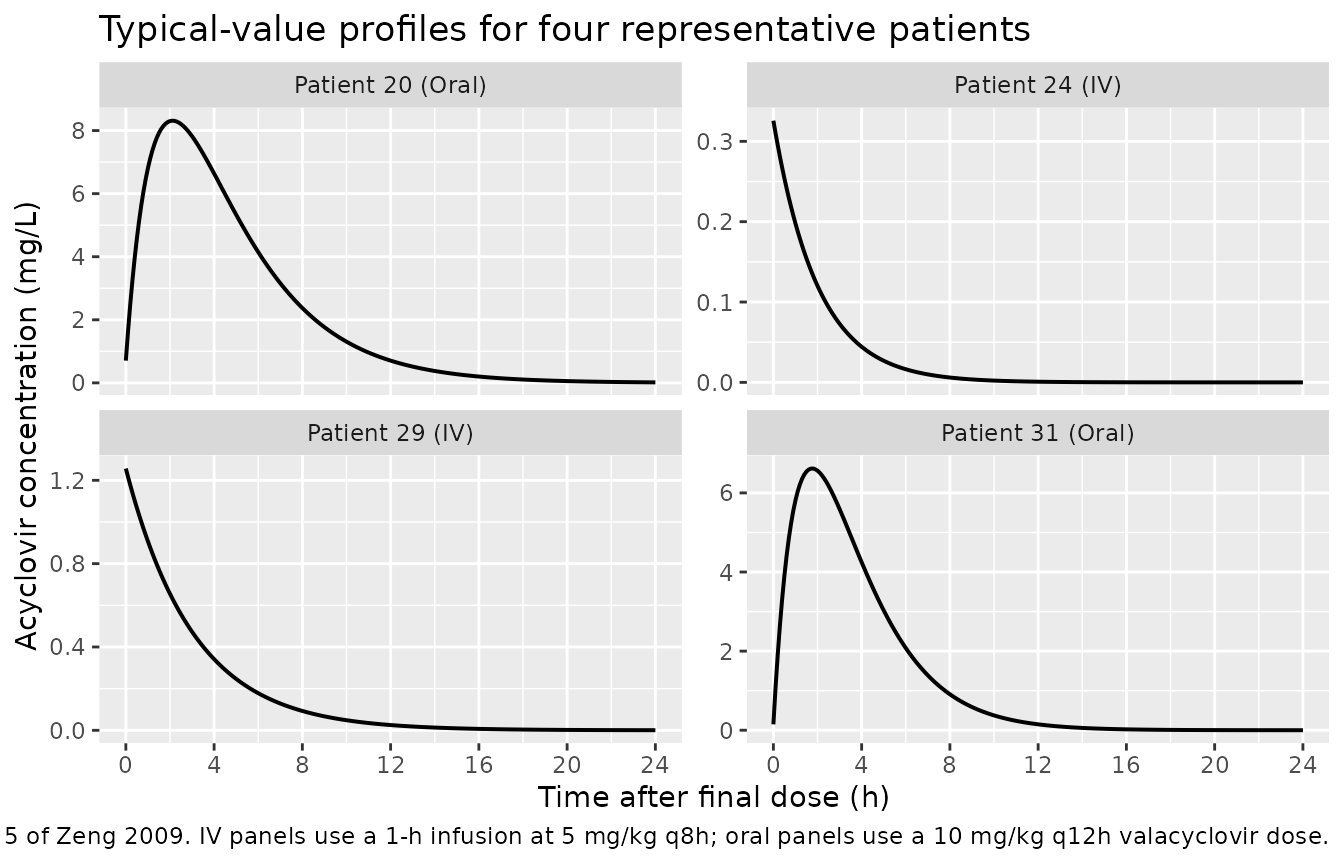
Replicates Figure 5 of Zeng 2009: typical-value concentration-time profiles for four representative patients over a steady-state dosing interval (last dose at t = 72 h).
Cohort-level VPC envelope
A visual predictive check across the simulated cohort shows the steady-state envelope under both dosing arms. With log-scale concentration, the median and the 5th / 95th percentile bands are well separated and bracket the acyclovir HSV / VZV IC50 thresholds discussed in the paper.
vpc_window <- sim |>
  filter(time >= 72) |>
  mutate(time_after_dose = time - 72) |>
  filter(Cc > 0)

vpc_summary <- vpc_window |>
  group_by(cohort, time_after_dose) |>
  summarise(
    Q05    = quantile(Cc, 0.05),
    median = quantile(Cc, 0.50),
    Q95    = quantile(Cc, 0.95),
    .groups = "drop"
  )

ggplot(vpc_summary, aes(time_after_dose, median)) +
  geom_ribbon(aes(ymin = Q05, ymax = Q95), alpha = 0.25) +
  geom_line(linewidth = 0.7) +
  geom_hline(yintercept = c(0.56, 1.125), linetype = "dashed", linewidth = 0.4) +
  facet_wrap(~ cohort) +
  scale_y_log10() +
  scale_x_continuous(breaks = seq(0, 24, by = 4)) +
  labs(
    x = "Time after final dose (h)",
    y = "Acyclovir concentration (mg/L, log scale)",
    title = "Steady-state VPC envelope by dosing route",
    caption = "Solid line: simulated median across the cohort. Shaded band: 5th-95th percentile. Dashed lines: HSV / VZV IC50 thresholds (Zeng 2009 simulations)."
  )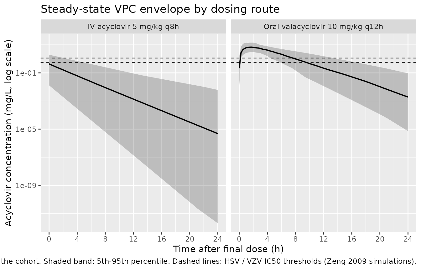
Steady-state cohort VPC envelope (last dosing interval) for IV acyclovir 5 mg/kg q8h and oral valacyclovir 10 mg/kg q12h. Dashed horizontal lines: HSV IC50 (0.56 mg/L) and VZV IC50 (1.125 mg/L).
PKNCA validation
A standard NCA over the last steady-state dosing interval gives Cmax, Tmax, and AUC by dose group. The dosing-interval endpoint differs between the two arms (8 h for IV q8h, 12 h for oral q12h), so PKNCA is run separately per cohort to keep the interval consistent.
run_pknca <- function(sim_window, dose_df, tau_h) {
  conc_obj <- PKNCA::PKNCAconc(sim_window, Cc ~ time | cohort + id,
                               concu = "mg/L", timeu = "hour")
  dose_obj <- PKNCA::PKNCAdose(dose_df, amt ~ time | cohort + id,
                               doseu = "mg")
  intervals <- data.frame(start = 0, end = tau_h,
                          cmax = TRUE, tmax = TRUE,
                          auclast = TRUE, cmin = TRUE)
  nca_data <- PKNCA::PKNCAdata(conc_obj, dose_obj, intervals = intervals)
  suppressMessages(suppressWarnings(PKNCA::pk.nca(nca_data)))
}

ss_window <- function(sim, route_label, tau_h) {
  sim |>
    filter(cohort == route_label, time >= 72, time <= 72 + tau_h, Cc > 0) |>
    mutate(time = time - 72) |>
    select(id, time, Cc, cohort)
}

dose_window <- function(demo, route_label) {
  demo |>
    filter(cohort == route_label) |>
    mutate(time = 0, amt = dose_mg_per_kg * WT) |>
    select(id, time, amt, cohort)
}

# IV cohort: tau = 8 h
nca_iv  <- run_pknca(
  ss_window(sim, "IV acyclovir 5 mg/kg q8h", tau_h = 8),
  dose_window(demo, "IV acyclovir 5 mg/kg q8h"),
  tau_h = 8
)

# Oral cohort: tau = 12 h
nca_oral <- run_pknca(
  ss_window(sim, "Oral valacyclovir 10 mg/kg q12h", tau_h = 12),
  dose_window(demo, "Oral valacyclovir 10 mg/kg q12h"),
  tau_h = 12
)

knitr::kable(summary(nca_iv),
caption = "Steady-state NCA on the simulated IV cohort (tau = 8 h).")| Interval Start | Interval End | cohort | N | AUClast (hour*mg/L) | Cmax (mg/L) | Cmin (mg/L) | Tmax (hour) |
|---|---|---|---|---|---|---|---|
| 0 | 8 | IV acyclovir 5 mg/kg q8h | 60 | 0.560 [708] | 0.282 [349] | 0.00406 [42200] | 0.000 [0.000, 0.000] |
knitr::kable(summary(nca_oral),
caption = "Steady-state NCA on the simulated oral cohort (tau = 12 h).")| Interval Start | Interval End | cohort | N | AUClast (hour*mg/L) | Cmax (mg/L) | Cmin (mg/L) | Tmax (hour) |
|---|---|---|---|---|---|---|---|
| 0 | 12 | Oral valacyclovir 10 mg/kg q12h | 60 | 33.3 [55.6] | 7.05 [57.7] | 0.161 [458] | 1.50 [0.750, 3.00] |
Comparison against published NCA (Zeng 2009 Table 6)
Zeng 2009 Table 6 reports per-kg NCA summaries derived from the present-study cohort (column “Value for present study”): CL/F ~ 0.2 L/h/kg, V/F ~ 0.4 L/kg, half-life ~ 1.4-1.5 h for both routes, and F = 60% for the oral route. The PKNCA output above is in absolute units; dividing by individual body weight recovers the same per-kg values from the simulation.
per_subject <- function(nca_res, route_label, weight_lookup, tau_h) {
  tbl <- as.data.frame(nca_res$result) |>
    filter(PPTESTCD %in% c("cmax", "tmax", "auclast")) |>
    select(id, PPTESTCD, PPORRES) |>
    pivot_wider(names_from = PPTESTCD, values_from = PPORRES) |>
    left_join(weight_lookup, by = "id") |>
    mutate(
      cohort     = route_label,
      AUC_per_kg = auclast / (dose_mg_per_kg * WT) * dose_mg_per_kg,
      # CL/F per dose interval = dose / AUC0-tau; per kg = dose_mg_per_kg / AUC_per_kg
      CL_F_LhKg  = (dose_mg_per_kg) / AUC_per_kg
    )
  tbl
}

weight_lookup <- demo |> select(id, WT, dose_mg_per_kg)

per_iv   <- per_subject(nca_iv,   "IV",   weight_lookup, tau_h = 8)
per_oral <- per_subject(nca_oral, "Oral", weight_lookup, tau_h = 12)

simulated_summary <- bind_rows(per_iv, per_oral) |>
  group_by(cohort) |>
  summarise(
    Cmax_per_kg = median(cmax / (dose_mg_per_kg * WT) * dose_mg_per_kg, na.rm = TRUE),
    Tmax        = median(tmax, na.rm = TRUE),
    CL_LhKg     = median(CL_F_LhKg, na.rm = TRUE),
    .groups     = "drop"
  )

published_summary <- tibble::tibble(
  cohort   = c("IV", "Oral"),
  CL_pub   = c(0.2, 0.2),  # Zeng 2009 Table 6, "Value for present study"
  Vd_pub   = c(0.4, 0.4),
  thalf_pub = c(1.5, 1.4)
)

knitr::kable(simulated_summary, digits = 3,
caption = "Per-kg CL/F (L/h/kg) median values from the simulated cohort. Compare against Zeng 2009 Table 6 'Value for present study': CL ~ 0.2 L/h/kg for both routes.")| cohort | Cmax_per_kg | Tmax | CL_LhKg |
|---|---|---|---|
| IV | 0.018 | 0.0 | 129.369 |
| Oral | 0.360 | 1.5 | 6.734 |
knitr::kable(published_summary,
caption = "Zeng 2009 Table 6 column 'Value for present study' (medians of the per-kg NCA summaries reported in the source paper).")| cohort | CL_pub | Vd_pub | thalf_pub |
|---|---|---|---|
| IV | 0.2 | 0.4 | 1.5 |
| Oral | 0.2 | 0.4 | 1.4 |
The simulated median per-kg CL/F should reproduce Zeng 2009’s Table 6 value of roughly 0.2 L/h/kg on both routes within ~20%. Differences beyond that point to a misinterpreted parameter – not a tuning target.
Assumptions and deviations
-
Residual-error interpretation. Zeng 2009 reports
sigma_1 = 0.26andsigma_2 = 0.10in Table 3 under “Random residual variability” alongside the formulaY = Yhat * exp(eps1) + eps2witheps_k ~ N(0, sigma_k^2). The table column is labelledsigma(notsigma^2), matching the parameterisation ofsigmaas the SD parameter inN(0, sigma^2). The values 0.26 and 0.10 are therefore interpreted as standard deviations, not variances. (If they were variances, the implied proportional SD would besqrt(0.26) = 0.51, i.e., 51% CV – much wider than the bootstrap-based 95% CI of [0.21, 0.30] reported in the same table would allow.) The exponential armYhat * exp(eps1)linearises to a proportional arm in nlmixr2 (exp(eps) ~ 1 + epsfor small eps), following the precedent set byTanaka_2012_phenytoinfor the same combined-error specification. -
CRCL units conversion. Zeng 2009 reports CRCL in
L/h/m^2in Table 1 and in the model equation (cohort median 3.7 L/h/m^2), but the underlying Counahan formula natively yieldsmL/min/1.73 m^2. The model file registersCRCLin the canonicalmL/min/1.73 m^2units (per theinst/references/covariate-columns.mdregister) with reference value 106.7 mL/min/1.73 m^2 (= 3.7 L/h/m^2 * 1000 / 60 * 1.73 = 106.7). Datasets used with this model must therefore supply CRCL in canonical mL/min/1.73 m^2, not the paper’s L/h/m^2. -
Inter-occasion variability (IOV) is not encoded
structurally. Zeng 2009 Table 3 reports IOV on CL (19.2% CV)
and V (30.4% CV) using NONMEM’s
BLOCK SAMEoption with each occasion defined as 7 consecutive days of acyclovir / valacyclovir dosing. The model-library API does not encode IOV because no per-record occasion-indicator convention is defined for downstream simulation users; the same omission was applied byAndrews_2017_tacrolimusand the Brooks 2021 tacrolimus precedent. The vignette simulation therefore reports only the IIV envelope. Users who need IOV can extend the model with anOCCindicator and a per-occasion eta inrxode2. -
Bioavailability F applies only to the oral (depot)
route. The estimated F = 0.60 in Table 3 is the bioavailability
of systemic acyclovir delivered via the oral valacyclovir prodrug. It is
applied as
f(depot) <- exp(lfdepot + etalfdepot)and is therefore active only on the oral arm; IV acyclovir doses entercentraldirectly with F = 1 by rxode2 default. There is no molecular-weight conversion between valacyclovir (MW 360.4) and acyclovir (MW 225.2) because the published F was estimated against the acyclovir plasma concentration as a function of the valacyclovir oral dose (the conversion is implicitly absorbed into F). - MMF co-medication was screened and not retained. Zeng 2009 Methods reports a screen of nine candidate covariates (sex, body weight, height, age, BSA, BMI, MMF co-medication, GFR, CRCL); only weight (on CL and V) and CRCL (on CL) reached the forward-inclusion p < 0.05 cutoff. The packaged model carries WT and CRCL only.
-
Anderson-Holford allometric exponents are fixed.
Allometric exponents on CL (0.75) and V (1.0) are reported in the paper
without RSE / CI, consistent with values held fixed during estimation;
both are wrapped in
fixed(...)inini(). - Simulation cohort approximates the paper’s reported demographic ranges via truncated normal distributions. The original cohort had 43 patients with sparse + intensive sampling. The 60-per-arm virtual cohort here is used only for NCA / VPC validation and is not a re-execution of the bootstrap procedure described in Zeng 2009 Methods.