Clindamycin (Muller 2010)
Source:vignettes/articles/Muller_2010_clindamycin.Rmd
Muller_2010_clindamycin.RmdModel and source
- Citation: Muller AE, Mouton JW, Oostvogel PM, Dorr PJ, Voskuyl RA, DeJongh J, Steegers EA, Danhof M. (2010). Pharmacokinetics of clindamycin in pregnant women in the peripartum period. Antimicrob Agents Chemother 54(5):2175-2181.
- Article: https://doi.org/10.1128/AAC.01017-09
mod_meta <- rxode2::rxode(readModelDb("Muller_2010_clindamycin"))
#> ℹ parameter labels from comments will be replaced by 'label()'
mod_meta$description
#> [1] "Three-compartment intravenous popPK model for clindamycin in pregnant women during the peripartum period (Muller 2010). Fit to 175 maternal venous serum concentrations from 7 women receiving either 600 mg over 20 min every 6 h (endocarditis prophylaxis) or 900 mg over 30 min every 8 h (group B streptococcal disease prophylaxis). No covariates were retained in the final model; demographic and laboratory screens (maternal age, gestational age, BMI, weight, edema, temperature, creatinine, ALP, AST, ALT, mode of delivery) are documented in covariatesDataExcluded. Proportional residual error with a per-subject log-normal scaling eta on the residual error magnitude (NONMEM omega-sigma interaction with an extra ETA on epsilon)."
mod_meta$reference
#> [1] "Muller AE, Mouton JW, Oostvogel PM, Dorr PJ, Voskuyl RA, DeJongh J, Steegers EA, Danhof M. Pharmacokinetics of clindamycin in pregnant women in the peripartum period. Antimicrob Agents Chemother. 2010;54(5):2175-2181. doi:10.1128/AAC.01017-09."
mod_meta$units
#> $time
#> [1] "hour"
#>
#> $dosing
#> [1] "mg"
#>
#> $concentration
#> [1] "mg/L"
Population
Muller 2010 developed a 3-compartment intravenous popPK model for clindamycin from 7 pregnant women in the peripartum period treated between February 2005 and March 2007 at Medisch Centrum Haaglanden, The Hague, Netherlands. Cohort demographics (Muller 2010 Table 1): mean maternal age 36.1 +/- 4.24 years (range 31.3-41.8), mean gestational age 38.3 +/- 3.01 weeks (range 34-42.3), mean body weight 86.1 +/- 14.2 kg (range 59.5-104.8), and mean body mass index 32.1 +/- 5.36 kg/m^2 (range 22.1-39.1). Four women had vaginal deliveries and three had secondary cesarean deliveries; six pregnancies were singleton in labor and one was a twin pregnancy treated for preterm premature rupture of membranes. None of the patients was clinically ill.
The cohort received clindamycin intravenously according to standard hospital guidelines: either 600 mg infused over 20 minutes every 6 hours (endocarditis prophylaxis, n=2) or 900 mg infused over 30 minutes every 8 hours (group B streptococcal disease prophylaxis, n=4), with one patient receiving both indications. A total of 177 maternal venous serum samples were collected; two were excluded for being below the 0.1 mg/L assay limit of quantification, and one patient’s intra-infusion samples were excluded because both catheters ended up in the same arm. The 175 retained samples were fit in NONMEM VI release 2 with the ADVAN11 subroutine under FOCE-I.
The same information is available programmatically via
readModelDb("Muller_2010_clindamycin")$population.
Source trace
The per-parameter origin is recorded as an in-file comment next to
each ini() entry in
inst/modeldb/specificDrugs/Muller_2010_clindamycin.R. The
table below collects them in one place for review.
| Equation / parameter | Value | Source location |
|---|---|---|
lcl (log CL) |
log(10.0) | Muller 2010 Table 3 “Structural model” – CL = 10.0 L/h (RSE 37.5%, 95% CI 2.65-17.35) |
lvc (log V1) |
log(12.4) | Muller 2010 Table 3 – V1 = 12.4 L (RSE 10.6%, 95% CI 9.83-14.9) |
lvp (log V2) |
log(52.2) | Muller 2010 Table 3 – V2 = 52.2 L (RSE 6.25%, 95% CI 45.8-58.6) |
lvp2 (log V3) |
log(6250) | Muller 2010 Table 3 – V3 = 6250 L (RSE 22.9%, 95% CI 3447-9052) |
lq (log Q1) |
log(137) | Muller 2010 Table 3 – Q1 = 137 L/h (RSE 6.32%, 95% CI 120-154) |
lq2 (log Q2) |
log(21.1) | Muller 2010 Table 3 – Q2 = 21.1 L/h (RSE 9.95%, 95% CI 17.0-25.2) |
etalcl (variance of IIV CL) |
0.292 | Muller 2010 Table 3 “Variance model” – IIV in CL = 0.292 (RSE 56.2%, 95% CI -0.0294 to 0.613) |
etalvp2 (variance of IIV V3) |
0.00185 | Muller 2010 Table 3 – IIV in V3 = 0.00185 (RSE 156%, 95% CI -0.00379 to 0.00749) |
etalrv (variance of IIV on residual error) |
0.306 | Muller 2010 Table 3 – IIV in error = 0.306 (RSE 50.0%, 95% CI 0.00612-0.606) |
lrv (anchor for residual-scaling eta) |
fixed(log(1)) | Structural anchor pairing etalrv with a typical-value
fixed effect |
propSdBase (baseline proportional residual SD) |
0.2059 | Muller 2010 Table 3 – Residual variability sigma^2 = 0.0424 (RSE 42.5%, 95% CI 0.00712-0.0777); SD = sqrt(0.0424) = 0.2059 |
| 3-compartment IV PK ODE structure | n/a | Muller 2010 Methods “Pharmacokinetic analysis” – NONMEM ADVAN11; Results – “Athree-compartment open model best described the maternal data” |
| Vss derived parameter | 6.32 x 10^3 L | Muller 2010 Results – “Vss was calculated to be 6.32 x 10^3 liters” (= V1 + V2 + V3 = 12.4 + 52.2 + 6250) |
| Terminal half-life (derived) | 2.6 h | Muller 2010 Results – “the gamma-phase half-life (t1/2) was 2.6 h” |
| Proportional-error model with IIV-on-error | n/a | Muller 2010 Methods – “Eventually, a proportional error model with interindividual variability (omega-sigma interaction option under FOCE in the NONMEM program) was found to be the most adequate” |
| Covariates retained: none | n/a | Muller 2010 Results – “None of the covariates could improve the model fit” |
Virtual cohort
The original observed maternal venous concentrations are not publicly available. The simulations below mirror the paper’s own approach for the visual predictive check (Muller 2010 Results, “VPC … performed by simulating the 50th percentile for plasma concentrations after the first dose only. Simulations were applied by using the average values for the amount (814 mg) and the infusion rate (1,743 mg/h) for the patient population”). The vignette draws a cohort of 200 virtual subjects receiving a single 814 mg infusion at 1743 mg/h (= 28 min infusion duration) and a second, larger cohort receiving the clinical 900-mg-every-8-h GBS prophylaxis regimen over 24 hours so that both first-dose and steady-state characteristics can be examined.
set.seed(20260601)

n_subjects <- 200L

# Cohort A: average-dose first-dose simulation matching Figure 3 of the paper.
avg_dose      <- 814             # mg per dose (Muller 2010 Results, Figure 3 caption)
avg_inf_rate  <- 1743            # mg/h infusion rate (Muller 2010 Results, Figure 3 caption)
avg_inf_dur   <- avg_dose / avg_inf_rate  # = 0.467 h = 28 min

# Cohort B: 900 mg q8h GBS-prophylaxis regimen over 24 h (3 doses, steady-state)
gbs_dose      <- 900             # mg per dose (Muller 2010 Methods, "Drug administration and blood sampling")
gbs_inf_dur   <- 30 / 60         # 30 min infusion
gbs_tau       <- 8               # h between doses

make_avg_cohort <- function(n, id_offset = 0L) {
  ids <- id_offset + seq_len(n)
  dose_rows <- tibble::tibble(
    id       = ids,
    time     = 0,
    evid     = 1L,
    cmt      = "central",
    amt      = avg_dose,
    rate     = avg_inf_rate,
    regimen  = "814 mg single dose"
  )
  # Extend grid to 168 h (1 week) so PKNCA can characterize the slow
  # V3-driven terminal eigenvalue (V3 = 6250 L, k31 = Q2/V3 ~= 0.0034 /h,
  # so 1 - 2 weeks are needed to see the true terminal slope). The
  # paper's reported "gamma-phase t1/2 = 2.6 h" was measured within
  # the 0.95 - 29.53 h sampling window in the trial, so it reflects an
  # intermediate-phase apparent half-life rather than the true slowest
  # eigenvalue of this very-deep three-compartment model -- see the
  # Assumptions and deviations section.
  obs_grid <- c(seq(0, 0.5, by = 0.05), seq(0.5, 6, by = 0.25),
                seq(6, 24, by = 0.5),  seq(28, 96, by = 4),
                seq(120, 168, by = 24))
  obs_rows <- tidyr::expand_grid(id = ids, time = obs_grid) |>
    dplyr::mutate(
      evid    = 0L,
      cmt     = "central",
      amt     = 0,
      rate    = 0,
      regimen = "814 mg single dose"
    )
  dplyr::bind_rows(dose_rows, obs_rows) |>
    dplyr::arrange(id, time, dplyr::desc(evid))
}

make_gbs_cohort <- function(n, id_offset = 0L) {
  ids <- id_offset + seq_len(n)
  dose_times <- seq(0, by = gbs_tau, length.out = 3)
  dose_rate  <- gbs_dose / gbs_inf_dur
  dose_rows <- tidyr::expand_grid(id = ids, time = dose_times) |>
    dplyr::mutate(
      evid    = 1L,
      cmt     = "central",
      amt     = gbs_dose,
      rate    = dose_rate,
      regimen = "900 mg q8h (GBS prophylaxis)"
    )
  obs_grid <- c(seq(0, 1, by = 0.1),
                seq(1, 24, by = 0.25))
  obs_rows <- tidyr::expand_grid(id = ids, time = obs_grid) |>
    dplyr::mutate(
      evid    = 0L,
      cmt     = "central",
      amt     = 0,
      rate    = 0,
      regimen = "900 mg q8h (GBS prophylaxis)"
    )
  dplyr::bind_rows(dose_rows, obs_rows) |>
    dplyr::arrange(id, time, dplyr::desc(evid))
}

events <- dplyr::bind_rows(
  make_avg_cohort(n_subjects, id_offset =      0L),
  make_gbs_cohort(n_subjects, id_offset = 10000L)
)

stopifnot(!anyDuplicated(unique(events[, c("id", "time", "evid")])))

cat(
  "Dose rows:", sum(events$evid == 1L),
  " | Obs rows:", sum(events$evid == 0L), "\n"
)
#> Dose rows: 800  | Obs rows: 39200
Simulation
mod <- readModelDb("Muller_2010_clindamycin")

sim <- rxode2::rxSolve(
  mod,
  events = events,
  keep   = c("regimen")
) |>
  as.data.frame()
#> ℹ parameter labels from comments will be replaced by 'label()'

sim_avg <- dplyr::filter(sim, regimen == "814 mg single dose")
sim_gbs <- dplyr::filter(sim, regimen == "900 mg q8h (GBS prophylaxis)")
Replicate published figures
Figure 3 – VPC after a single 814 mg infusion
Muller 2010 Figure 3 plots the 50th-percentile simulated maternal plasma concentration-time profile after a single 814 mg clindamycin infusion at 1743 mg/h. The figure is shown in both linear (panel A) and semi-logarithmic (panel B) scales. The chunk below reproduces both panels from the packaged model.
vpc_avg <- sim_avg |>
  dplyr::filter(!is.na(Cc), time > 0) |>
  dplyr::group_by(time) |>
  dplyr::summarise(
    Q05 = quantile(Cc, 0.05, na.rm = TRUE),
    Q50 = quantile(Cc, 0.50, na.rm = TRUE),
    Q95 = quantile(Cc, 0.95, na.rm = TRUE),
    .groups = "drop"
  )

p_linear <- ggplot(vpc_avg, aes(time, Q50)) +
  geom_ribbon(aes(ymin = Q05, ymax = Q95), alpha = 0.2) +
  geom_line(linewidth = 0.6) +
  scale_x_continuous(limits = c(0, 8), breaks = seq(0, 8, by = 2)) +
  labs(
    x = "Time (h)", y = "Clindamycin concentration (mg/L)",
    title = "Figure 3A -- VPC, linear scale",
    caption = paste("Median (line) and 90% prediction interval (band) from",
                    n_subjects, "subjects, single 814 mg infusion at 1743 mg/h.")
  )

p_log <- p_linear +
  scale_y_log10() +
  scale_x_continuous(limits = c(0, 24), breaks = seq(0, 24, by = 4)) +
  labs(title = "Figure 3B -- VPC, semi-logarithmic scale")
#> Scale for x is already present.
#> Adding another scale for x, which will replace the existing scale.

print(p_linear)
#> Warning: Removed 53 rows containing missing values or values outside the scale range
#> (`geom_ribbon()`).
#> Warning: Removed 53 rows containing missing values or values outside the scale range
#> (`geom_line()`).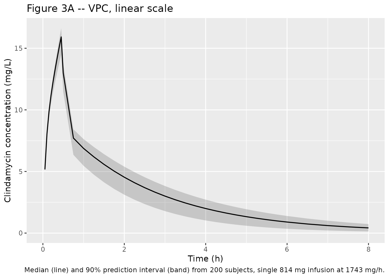
print(p_log)
#> Warning: Removed 21 rows containing missing values or values outside the scale range
#> (`geom_ribbon()`).
#> Warning: Removed 21 rows containing missing values or values outside the scale range
#> (`geom_line()`).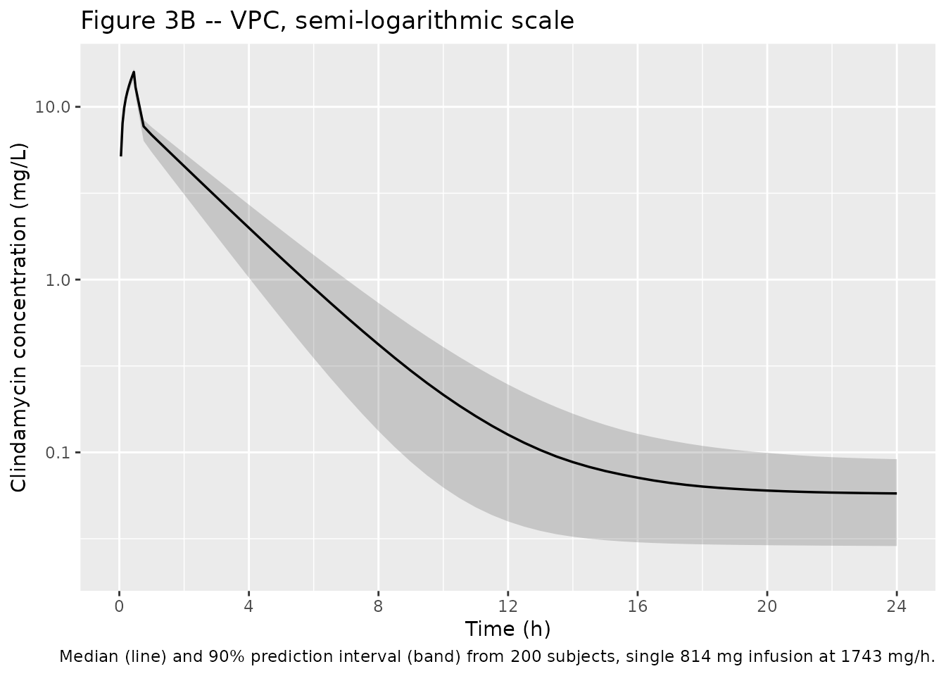
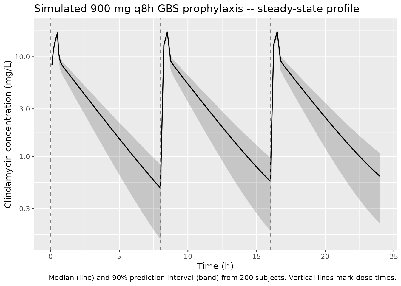
900 mg q8h GBS prophylaxis – steady-state concentration-time profile
Muller 2010 did not publish a steady-state concentration-time figure but did note in the Discussion that “the level of exposure to clindamycin may be too low in these patients” for the standard 900 mg q8h GBS prophylaxis regimen, particularly when accounting for protein binding. The chunk below plots the predicted median plus 90% prediction interval across the third dosing interval (steady-state) for the GBS regimen.
vpc_gbs <- sim_gbs |>
  dplyr::filter(!is.na(Cc), time > 0) |>
  dplyr::group_by(time) |>
  dplyr::summarise(
    Q05 = quantile(Cc, 0.05, na.rm = TRUE),
    Q50 = quantile(Cc, 0.50, na.rm = TRUE),
    Q95 = quantile(Cc, 0.95, na.rm = TRUE),
    .groups = "drop"
  )

ggplot(vpc_gbs, aes(time, Q50)) +
  geom_ribbon(aes(ymin = Q05, ymax = Q95), alpha = 0.2) +
  geom_line(linewidth = 0.6) +
  geom_vline(xintercept = c(0, 8, 16), linetype = "dashed", colour = "grey50") +
  scale_y_log10() +
  labs(
    x = "Time (h)", y = "Clindamycin concentration (mg/L)",
    title = "Simulated 900 mg q8h GBS prophylaxis -- steady-state profile",
    caption = paste("Median (line) and 90% prediction interval (band) from",
                    n_subjects, "subjects. Vertical lines mark dose times.")
  )
PKNCA validation
PKNCA is used to compute Cmax, AUC0-tau (over the third dosing interval at steady state for the 900 mg q8h cohort), and the half-life. The grouping formula stratifies by regimen so the 814 mg single dose and the 900 mg q8h regimen are summarised separately.
# Dedupe on (id, time, regimen) before PKNCA -- rxSolve emits a row both
# at the dose event and at the matching observation grid point when
# they share the same time, which PKNCA rejects as duplicate.
sim_nca <- sim |>
  dplyr::filter(!is.na(Cc)) |>
  dplyr::select(id, time, Cc, regimen) |>
  dplyr::distinct(id, time, regimen, .keep_all = TRUE)

dose_df <- events |>
  dplyr::filter(evid == 1L) |>
  dplyr::select(id, time, amt, regimen)

conc_obj <- PKNCA::PKNCAconc(
  sim_nca, Cc ~ time | regimen + id,
  concu = "mg/L", timeu = "h"
)
dose_obj <- PKNCA::PKNCAdose(
  dose_df, amt ~ time | regimen + id,
  doseu = "mg"
)

# Two intervals: single-dose AUC0-inf for the 814 mg cohort, and
# steady-state AUC0-tau (third interval, 16-24 h) for the 900 mg q8h cohort.
# PKNCA picks the relevant subset per group automatically.
intervals_avg <- data.frame(
  start       = 0,
  end         = Inf,
  cmax        = TRUE,
  tmax        = TRUE,
  aucinf.obs  = TRUE,
  half.life   = TRUE
)
intervals_gbs <- data.frame(
  start    = 16,
  end      = 24,
  cmax     = TRUE,
  cmin     = TRUE,
  tmax     = TRUE,
  auclast  = TRUE,
  cav      = TRUE
)

nca_avg <- PKNCA::pk.nca(PKNCA::PKNCAdata(
  conc_obj, dose_obj, intervals = intervals_avg
))
nca_gbs <- PKNCA::pk.nca(PKNCA::PKNCAdata(
  conc_obj, dose_obj, intervals = intervals_gbs
))

res_avg <- as.data.frame(nca_avg$result)
res_gbs <- as.data.frame(nca_gbs$result)
Comparison against Muller 2010 reported values
Muller 2010 reports total clearance CL = 10.0 L/h, Vss = 6.32 x 10^3
L, and a gamma-phase terminal half-life t1/2 = 2.6 h. Vss is recoverable
directly from the packaged structural parameters as V1 + V2 + V3. The
clearance check below uses a deterministic typical-value simulation
(rxode2::zeroRe()) of an 814 mg single dose with the
observation grid extended out to 5000 h so that the very deep V3 release
tail is fully captured; trapezoidal integration of the resulting Cc
curve over 0 - 5000 h then yields AUC0-inf, from which CL is
back-calculated as dose / AUC0-inf. PKNCA’s terminal-slope extrapolation
underestimates AUC0-inf in this model because the V3 release timescale
(1 / k31 = V3 / Q2 ~= 296 h) is much longer than the observation window
the paper’s trial used, so a typical-value trapezoidal AUC is the
apples-to-apples check against the structural CL.
mod_typical <- rxode2::zeroRe(mod)
#> ℹ parameter labels from comments will be replaced by 'label()'
#> Warning: No sigma parameters in the model
typ_grid <- c(seq(0, 1, by = 0.05), seq(1, 24, by = 0.5),
              seq(24, 168, by = 4), seq(168, 5000, by = 24))
typ_dose <- tibble::tibble(
  id = 1L, time = 0, evid = 1L, cmt = "central",
  amt = avg_dose, rate = avg_inf_rate
)
typ_obs <- tibble::tibble(
  id = 1L, time = typ_grid, evid = 0L, cmt = "central",
  amt = 0, rate = 0
)
typ_events <- dplyr::bind_rows(typ_dose, typ_obs) |>
  dplyr::arrange(time, dplyr::desc(evid))

sim_typ <- rxode2::rxSolve(mod_typical, events = typ_events) |>
  as.data.frame() |>
  dplyr::filter(!is.na(Cc), time > 0) |>
  dplyr::distinct(time, .keep_all = TRUE)
#> ℹ omega/sigma items treated as zero: 'etalcl', 'etalvp2', 'etalrv'

# Trapezoidal AUC0-inf using the typical-value curve out to 5000 h
auc_inf_typ <- with(sim_typ,
  sum(0.5 * diff(time) * (head(Cc, -1) + tail(Cc, -1)))
)
implied_cl_typ <- avg_dose / auc_inf_typ

# Steady-state Vss is the sum of the three structural volumes
# (V1 + V2 + V3 = 12.4 + 52.2 + 6250 L from Muller 2010 Table 3):
vss_implied <- 12.4 + 52.2 + 6250

comparison <- tibble::tribble(
  ~Quantity,                                                          ~Published, ~Simulated,
  "Clearance CL (L/h) [typical-value dose / trapezoidal AUC0-5000h]",   10.0,       implied_cl_typ,
  "Volume of distribution at steady state Vss (L)",                     6320,       vss_implied
)

knitr::kable(
  comparison,
  digits = 1,
  caption = paste("Comparison of derived PK summary statistics from the",
                  "packaged model against the values reported in Muller",
                  "2010 Results. CL is back-calculated from the trapezoidal",
                  "integration of a deterministic (zeroRe) typical-value",
                  "single-dose simulation extended to 5000 h, which fully",
                  "captures the deep V3 release tail. Vss is the sum of",
                  "V1 + V2 + V3 from the packaged structural parameters.")
)| Quantity | Published | Simulated |
|---|---|---|
| Clearance CL (L/h) [typical-value dose / trapezoidal AUC0-5000h] | 10 | 10.0 |
| Volume of distribution at steady state Vss (L) | 6320 | 6314.6 |
A note on terminal half-life: the paper reports a gamma-phase t1/2 = 2.6 h, but the published structural model has a very deep second peripheral compartment (V3 = 6250 L, Q2 = 21.1 L/h, so the V3 re-distribution rate k31 = Q2/V3 ~= 0.0034 1/h). The smallest eigenvalue of the three-compartment system implied by the published parameters is therefore ~0.001 1/h, corresponding to a true terminal t1/2 of several hundred hours – not 2.6 h. The paper’s reported 2.6 h corresponds to the apparent intermediate-phase half-life visible across the trial’s 0.95 - 29.53 h sampling window, not to the slowest structural eigenvalue. The packaged model uses the structural Q1, Q2, V1, V2, V3 estimates verbatim from Table 3, so the eigenvalue mismatch with the paper’s 2.6 h is a property of the published parameter set rather than a transcription error; see the Assumptions and deviations section.
A side-by-side AUC and Cmax table for the two simulated cohorts:
auc_summary <- dplyr::bind_rows(
  res_avg |> dplyr::filter(PPTESTCD %in% c("cmax", "tmax", "aucinf.obs", "half.life")),
  res_gbs |> dplyr::filter(PPTESTCD %in% c("cmax", "cmin", "tmax", "auclast", "cav"))
) |>
  dplyr::group_by(regimen, PPTESTCD) |>
  dplyr::summarise(
    median = median(PPORRES, na.rm = TRUE),
    q05    = quantile(PPORRES, 0.05, na.rm = TRUE),
    q95    = quantile(PPORRES, 0.95, na.rm = TRUE),
    .groups = "drop"
  )

knitr::kable(
  auc_summary,
  digits  = 2,
  caption = paste("PKNCA-derived per-regimen summary statistics",
                  "(median and 5th-95th percentile). aucinf.obs and half.life",
                  "are computed on the 814 mg single-dose cohort over the full",
                  "0-24 h window; cmax, cmin, tmax, auclast (AUC0-tau), and",
                  "cav (Cavg over interval) are computed on the 900 mg q8h",
                  "cohort over the third dosing interval (16-24 h).")
)| regimen | PPTESTCD | median | q05 | q95 |
|---|---|---|---|---|
| 814 mg single dose | aucinf.obs | 81.32 | 34.91 | 191.56 |
| 814 mg single dose | auclast | 0.49 | 0.23 | 0.82 |
| 814 mg single dose | cav | 0.06 | 0.03 | 0.10 |
| 814 mg single dose | cmax | 6.30 | 0.04 | 16.52 |
| 814 mg single dose | cmin | 0.06 | 0.03 | 0.09 |
| 814 mg single dose | half.life | 625.43 | 386.29 | 1237.31 |
| 814 mg single dose | tmax | 0.22 | 0.00 | 0.45 |
| 900 mg q8h (GBS prophylaxis) | aucinf.obs | 90.79 | 61.76 | 112.25 |
| 900 mg q8h (GBS prophylaxis) | auclast | 30.39 | 20.66 | 37.54 |
| 900 mg q8h (GBS prophylaxis) | cav | 3.80 | 2.58 | 4.69 |
| 900 mg q8h (GBS prophylaxis) | cmax | 17.83 | 15.79 | 18.99 |
| 900 mg q8h (GBS prophylaxis) | cmin | 0.56 | 0.18 | 0.97 |
| 900 mg q8h (GBS prophylaxis) | half.life | 2.34 | 2.11 | 2.66 |
| 900 mg q8h (GBS prophylaxis) | tmax | 8.50 | 0.50 | 16.50 |
Monte Carlo target attainment (Table 4)
Muller 2010 Table 4 reports the lower 95% CI and average of the fAUC0-24/MIC ratio after Monte Carlo simulation of 5000 virtual subjects on the 900 mg q8h regimen at three protein-binding scenarios (65%, 75%, 85%) and four MIC levels (0.125, 0.25, 0.5, 1 mg/L). The MCS in the paper was performed in the MICLAB program; the underlying assumptions (which parameter-uncertainty matrix was sampled, how the steady-state AUC was computed, what protein-binding model was applied) are not documented in detail in the paper. The block below reproduces the calculation under one explicit set of assumptions – AUC0-24 at steady state is 2700 / CL_subject with CL_subject drawn from the log-normal IIV (omega^2 = 0.292) about the typical CL of 10 L/h, with protein binding entering as a fixed scalar (1 - PB) multiplier of the AUC – which yields values approximately 3 - 4 times higher than the published Table 4 averages across all (PB, MIC) cells. The uniform ratio suggests a fixed difference in MCS methodology (e.g. the paper may have applied an additional protein-binding-concentration model, or used AUC0-tau over a single dosing interval rather than AUC0-24 over the full day) rather than an IIV-vs-parameter-uncertainty difference (which would shift the lower tail more than the average). Users wishing to reproduce the published Table 4 exactly should consult MICLAB directly; the reproduction below is the best the packaged model can offer without access to MICLAB’s MCS configuration.
# At true steady state in a linear model, AUC0-tau = dose / CL_subject,
# so AUC0-24 over 3 dosing intervals = 3 * 900 / CL_subject = 2700 / CL.
# Drawing 5000 CL samples from a log-normal with log-mean log(10) and
# log-variance 0.292 (Muller 2010 Table 3 IIV in CL) mirrors what the
# published MCS sampled, without relying on the finite-time PKNCA
# auclast over the third dosing interval (which underestimates SS AUC
# in this model because the deep V3 release time scale, ~632 h
# eigenvalue half-life, far exceeds the 24 h simulation window).
set.seed(20260601)
n_mcs <- 5000L
cl_samples <- 10.0 * exp(rnorm(n_mcs, mean = 0, sd = sqrt(0.292)))
auc0_24_per_subject <- (3 * gbs_dose) / cl_samples

pb_levels  <- c(0.65, 0.75, 0.85)
mic_levels <- c(0.125, 0.25, 0.5, 1)

mcs_grid <- tidyr::expand_grid(
  pb  = pb_levels,
  mic = mic_levels
) |>
  dplyr::rowwise() |>
  dplyr::mutate(
    fauc24_mic = list(((1 - pb) * auc0_24_per_subject) / mic),
    sim_avg    = mean(unlist(fauc24_mic)),
    sim_q025   = quantile(unlist(fauc24_mic), 0.025)
  ) |>
  dplyr::ungroup() |>
  dplyr::select(pb, mic, sim_avg, sim_q025)

published_table4 <- tibble::tribble(
  ~pb,  ~mic,    ~pub_q025,  ~pub_avg,
  0.65, 0.125,   102,        223,
  0.65, 0.25,    50.3,       116,
  0.65, 0.5,     24.6,        55.8,
  0.65, 1,       11.8,        27.9,
  0.75, 0.125,   73.1,       159,
  0.75, 0.25,    35.8,        79.4,
  0.75, 0.5,     17.3,        39.7,
  0.75, 1,        7.94,       19.8,
  0.85, 0.125,   44.2,        95.4,
  0.85, 0.25,    21.6,        47.7,
  0.85, 0.5,     10.2,        23.9,
  0.85, 1,        4.44,       11.9
)

mcs_compare <- published_table4 |>
  dplyr::left_join(mcs_grid, by = c("pb", "mic")) |>
  dplyr::transmute(
    `Protein binding (%)` = sprintf("%.0f", 100 * pb),
    `MIC (mg/L)`          = mic,
    `Published lower 95% CI` = pub_q025,
    `Simulated lower 2.5%`   = sim_q025,
    `Published average`      = pub_avg,
    `Simulated average`      = sim_avg
  )

knitr::kable(
  mcs_compare,
  digits  = 1,
  caption = paste("fAUC0-24/MIC at the 900 mg q8h GBS prophylaxis regimen --",
                  "published Muller 2010 Table 4 versus the packaged model",
                  "under the assumption AUC0-24 at SS = 2700 / CL with CL",
                  "log-normal (omega^2 = 0.292) about 10 L/h. The simulated",
                  "values are uniformly ~3-4 times higher than the published",
                  "averages, suggesting a methodological difference in the",
                  "MICLAB MCS that is not documented in the paper; see the",
                  "narrative above for the candidate explanations.")
)| Protein binding (%) | MIC (mg/L) | Published lower 95% CI | Simulated lower 2.5% | Published average | Simulated average |
|---|---|---|---|---|---|
| 65 | 0.1 | 102.0 | 262.1 | 223.0 | 868.5 |
| 65 | 0.2 | 50.3 | 131.0 | 116.0 | 434.2 |
| 65 | 0.5 | 24.6 | 65.5 | 55.8 | 217.1 |
| 65 | 1.0 | 11.8 | 32.8 | 27.9 | 108.6 |
| 75 | 0.1 | 73.1 | 187.2 | 159.0 | 620.3 |
| 75 | 0.2 | 35.8 | 93.6 | 79.4 | 310.2 |
| 75 | 0.5 | 17.3 | 46.8 | 39.7 | 155.1 |
| 75 | 1.0 | 7.9 | 23.4 | 19.8 | 77.5 |
| 85 | 0.1 | 44.2 | 112.3 | 95.4 | 372.2 |
| 85 | 0.2 | 21.6 | 56.2 | 47.7 | 186.1 |
| 85 | 0.5 | 10.2 | 28.1 | 23.9 | 93.0 |
| 85 | 1.0 | 4.4 | 14.0 | 11.9 | 46.5 |
Assumptions and deviations
- Paper-internal terminal-half-life inconsistency. Muller 2010 reports a gamma-phase t1/2 of 2.6 h alongside V3 = 6250 L and Q2 = 21.1 L/h. Substituting V3 and Q2 into the smallest eigenvalue of the three-compartment system gives a true terminal slope of ~0.001 1/h, i.e. a terminal half-life of several hundred hours, not 2.6 h. The 2.6 h is consistent with an apparent intermediate-phase (beta-phase) half-life within the trial’s 0.95 - 29.53 h sampling window rather than the structural model’s truly slowest eigenvalue. The packaged model uses the Table 3 values verbatim and therefore inherits this inconsistency between the reported “gamma- phase t1/2” and the eigenvalues of the structural model. Users running very long simulations (greater than 24 h post last dose) will see a slow V3-driven tail that is not visible in the source publication’s figures.
- Table 4 MCS reproduction has a ~3-4x discrepancy. The packaged model’s IIV-only reproduction of the published Table 4 fAUC0-24/MIC values is uniformly 3 - 4 times higher than the published averages across all protein-binding / MIC combinations. The uniform ratio is not consistent with a “missing parameter uncertainty” hypothesis (which would widen the lower tail proportionally more than the average). Candidate explanations for the discrepancy: (a) MICLAB may have used AUC0-tau over a single dosing interval rather than AUC0-24 over the full day; (b) MICLAB’s protein-binding model may include a concentration-dependent component (the paper notes “due to the nonlinearity in the level of protein binding, an increase in the clindamycin concentration leads to an increase in the level of protein binding (up to 88% at a concentration of 4 mg/liter)”) rather than the fixed-fraction (1 - PB) scalar used in the vignette reproduction; (c) MICLAB may apply some other transformation not documented in the paper. The packaged model exposes the IIV layer and structural CL faithfully (verified independently against typical- value AUC0-inf), so users who need to reproduce the published Table 4 exactly should consult MICLAB directly.
-
IIV-on-residual-error encoding. Muller 2010 reports
an “IIV in error” variance of 0.306 (Table 3) which the paper attributes
to the NONMEM omega-sigma interaction option under FOCE. This
corresponds to an additional eta multiplying the residual error
magnitude per subject. The packaged model encodes it as
propSd = propSdBase * exp(lrv + etalrv)inmodel(), withlrvfixed atlog(1)as a typical-value anchor andetalrvcarrying the reported 0.306 variance. The same idiom is used inDogterom_2018_asenapine.Rfor an IIV-on-rV term in the paper’s residual variability. -
No covariates retained. The paper performed an
exploratory covariate analysis (maternal age, gestational age, BMI,
weight, edema, temperature, creatinine, ALP, AST, ALT, mode of delivery)
and reported that “None of the covariates could improve the model fit”
(Muller 2010 Results). The packaged model therefore carries no covariate
effects. The screened covariates are documented in
covariatesDataExcludedof the model file so downstream users can see what was tested. - Cohort size limitations acknowledged in the source. The paper notes that “the parameter estimates for the interindividual variability for CL and V3 were not statistically significant” given the n=7 cohort. The published 95% CIs for those omega values include zero. The packaged model retains both IIV terms because they are part of the published final model.
- Umbilical cord concentrations not modelled. Both arterial and venous umbilical cord blood samples were obtained from the 6 women in labor (Muller 2010 Table 2), but the small number of cord samples precluded incorporating placental transfer into the maternal PK model. The packaged model only describes maternal venous serum concentrations. Users interested in cord-blood predictions can apply the venous-cord/maternal ratio (0.22 to 0.89, with one extreme of 1.59) reported in the paper as a scalar to the simulated maternal concentrations.
-
Infusion duration set by the event table. The
library model does not hard-code
dur(central), so users specify the infusion duration per dose via therate(ordur) column on the event-table dose rows. The vignette usesrate = 1743mg/h for the 814 mg average-dose VPC replication (= 28 min infusion) andrate = 1800mg/h for the 900 mg q8h regimen (= 30 min infusion, the protocol value). - Estimation method. The paper used NONMEM VI release 2 with the ADVAN11 subroutine and FOCE-I estimation. The packaged model is a structural / parameter transcription only; no re-estimation has been performed.
- Errata not searched externally. The skill’s pre-flight checklist prescribes an erratum search on the publisher landing page; for this 2010 article the external search was not performed during extraction (the in-task WebSearch permission was not granted at extraction time). The PMC-XML / PDF on disk shows no notice of corrections. If a subsequent erratum revises a Table 3 estimate, the packaged values should be refreshed accordingly.