Midazolam in rats on ECMO (Sato 2025)
Source:vignettes/articles/Sato_2025_midazolam_rat.Rmd
Sato_2025_midazolam_rat.RmdModel and source
- Citation: Sato Y, Motoishi E, Kakuba R, Nagatsuka Y, Abe T, Fujii Y. Pharmacokinetics of midazolam and hepatic cytochrome P450 3A activity in an in vivo extracorporeal membrane oxygenation rat model. Sci Rep. 2025;15:19363. doi:10.1038/s41598-025-03949-x.
- Description: Preclinical (rat). Two-compartment population PK model for intravenous bolus midazolam in anaesthetised male Sprague-Dawley rats with or without extracorporeal membrane oxygenation (ECMO) (Sato 2025). The only retained covariate is a binary ECMO indicator that multiplies the central volume 3.02-fold; clearance, the peripheral volume and the intercompartmental clearance are shared by both groups. Parameters are absolute (L, L/h) for 400-450 g rats, not per kilogram.
- Article: https://doi.org/10.1038/s41598-025-03949-x (open access)
Sato et al. gave a single 400 ug/kg intravenous bolus of midazolam to anaesthetised, mechanically ventilated male Sprague-Dawley rats, three of which were then placed on extracorporeal membrane oxygenation (ECMO) 2 min after the dose while three sham-operated rats served as controls. Plasma midazolam was measured for 180 min and fitted with a two-compartment population PK model in NONMEM. ECMO was the only covariate tested; it was retained as a 3.02-fold multiplier on the central volume. The paper also reports lower hepatic CYP3A (testosterone 6-beta-hydroxylation) activity in ECMO-treated livers; that in-vitro measurement is not part of the PK model.
Population
Twelve male Sprague-Dawley rats (14-16 weeks old, 400-450 g) were used; six of them formed the midazolam PK study, three on ECMO and three sham-operated (Methods, Experimental design). ECMO drained the right internal jugular vein and returned blood through the left common carotid artery cannula at an auxiliary flow of 60-70 mL/kg/min; the circuit was primed with 7 mL saline and 1 mL heparin (Supplementary Information 2). Forty-eight plasma samples were collected at eight times: 2 min after the dose (before ECMO started) and 5-180 min after ECMO initiation (Results, PK analysis).
The same information is available programmatically via
readModelDb("Sato_2025_midazolam_rat")()$population.
Source trace
| Equation / parameter | Value | Source location |
|---|---|---|
lcl (CL) |
log(0.69 L/h) | Table 3, theta CL (RSE 18.0%) |
lvc (V1, sham) |
log(0.22 L) | Table 3, theta V1 (RSE 41.2%) |
lvp (V2) |
log(0.49 L) | Table 3, theta V2 (RSE 34.4%) |
lq (Q) |
log(0.29 L/h) | Table 3, theta Q (RSE 20.5%) |
e_ecmo_status_vc |
3.02 | Table 3, dic (ECMO) (RSE 41.7%); assigned to V1 by the Results text and the Discussion (‘an increase in V1 (0.66 vs. 0.22 L)’) |
etalcl |
0.617 = log(0.924^2 + 1) | Table 3, omega CL = 92.4 CV% |
etalvc |
0.216 = log(0.491^2 + 1) | Table 3, omega V1 = 49.1 CV% |
propSd |
0.395 | Table 3, proportional residual = 39.5% |
IIV model theta_i = theta * exp(eta_i)
|
n/a | Methods, PK analysis, first equation |
Covariate model
theta_i = theta_pop * dic^ECMO * exp(eta_i)
|
n/a | Methods, PK analysis, third equation (see Assumptions) |
Residual model Y_obs = Y_pred * (1 + eps_prop)
|
n/a | Methods, PK analysis, second equation; Results (‘two-compartment model with a proportional error’) |
d/dt(central), d/dt(peripheral1)
|
n/a | Two-compartment model with V1, V2, CL, Q (Methods, PK analysis) |
Virtual cohort
The observed data are not public. Two virtual arms of 200 rats each (ECMO and sham) receive 400 ug/kg as an intravenous bolus. Body weight is drawn uniformly from the 400-450 g range of the paper and is used only to compute the dose in ug: the model’s volumes and clearances are absolute values for rats of that size, not per-kilogram parameters.
# One record per rat per sampling time. The observation grid runs to 3 h,
# the end of the paper's sampling, so that PKNCA sees the same window as the
# paper's NCA.
obs_times <- sort(unique(c(seq(0, 3, by = 1 / 12), c(2, 5, 15, 30, 45) / 60)))

make_arm <- function(n, ecmo, dose_ugkg, id_offset = 0L) {
  rats <- tibble(
    id = id_offset + seq_len(n),
    WT = runif(n, 0.400, 0.450),
    ECMO_STATUS = ecmo,
    group = if (ecmo == 1) "ECMO" else "Sham",
    amt = dose_ugkg * WT
  )
  doses <- rats |> mutate(time = 0, evid = 1L, cmt = "central")
  obs <- tidyr::expand_grid(rats |> select(-amt), time = obs_times) |>
    mutate(amt = 0, evid = 0L, cmt = "central")
  bind_rows(doses, obs) |> arrange(id, time, desc(evid))
}

set.seed(19363)
rxode2::rxSetSeed(19363)
events <- bind_rows(
  make_arm(200, ecmo = 1, dose_ugkg = 400, id_offset = 0L),
  make_arm(200, ecmo = 0, dose_ugkg = 400, id_offset = 200L)
)
stopifnot(!anyDuplicated(unique(events[, c("id", "time", "evid")])))
Simulation
mod <- readModelDb("Sato_2025_midazolam_rat")
sim <- rxode2::rxSolve(mod, events = events, keep = c("group", "WT")) |>
  as.data.frame()
#> ℹ parameter labels from comments will be replaced by 'label()'
Replicate published figures
Figure 3 and Figure 5: observed profiles against the model
The paper’s Figure 3 shows the mean +/- SD of the three rats per group and Figure 5 a 500-replicate VPC. The open circles below are the group means read off Figure 3 by the maintainers (approximate, to the resolution of the printed axis); the bands are the 5th-95th and 25th-75th percentiles of 200 simulated rats per group with the median as a line.
fig3_means <- tibble::tribble(
  ~group, ~time_min, ~Cc,
  "ECMO",   2, 395,
  "ECMO",   5, 243,
  "ECMO",  15, 185,
  "ECMO",  30, 142,
  "ECMO",  45,  90,
  "ECMO",  60,  97,
  "ECMO", 120,  78,
  "ECMO", 180,  62,
  "Sham",   2, 655,
  "Sham",   5, 390,
  "Sham",  15, 205,
  "Sham",  30, 132,
  "Sham",  45,  85,
  "Sham",  60,  60,
  "Sham", 120,  28,
  "Sham", 180,  15
) |>
  mutate(time = time_min / 60)

vpc <- sim |>
  group_by(group, time) |>
  summarise(
    Q05 = quantile(Cc, 0.05), Q25 = quantile(Cc, 0.25),
    Q50 = quantile(Cc, 0.50), Q75 = quantile(Cc, 0.75),
    Q95 = quantile(Cc, 0.95),
    .groups = "drop"
  )

ggplot(vpc, aes(time, Q50)) +
  geom_ribbon(aes(ymin = Q05, ymax = Q95), alpha = 0.15) +
  geom_ribbon(aes(ymin = Q25, ymax = Q75), alpha = 0.3) +
  geom_line() +
  geom_point(data = fig3_means, aes(time, Cc), shape = 1, size = 2) +
  facet_wrap(~group) +
  scale_y_log10() +
  labs(
    x = "Time after midazolam (h)", y = "Midazolam (ng/mL)",
    caption = "Replicates Figures 3 and 5 of Sato 2025 (400 ug/kg IV bolus)."
  )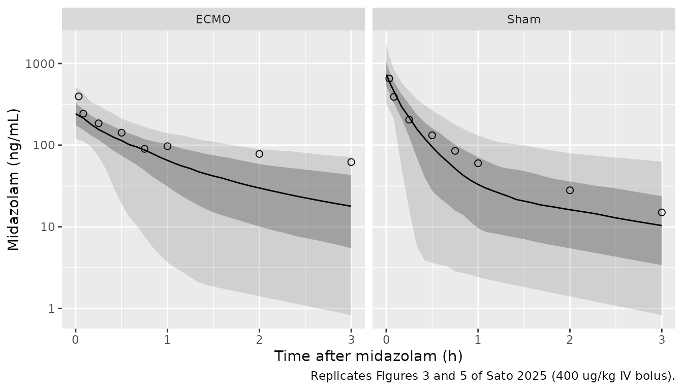
Up to about 45 min the observed means of both groups lie near the simulated median (at 15 min, for example, 205 vs about 220 ng/mL in the sham group and 185 vs about 155 ng/mL with ECMO). The late ECMO means (2-3 h) sit near the simulated 95th percentile: the final model carries no ECMO effect on clearance, so it does not reproduce the slower terminal decline the authors saw in the ECMO arm by noncompartmental analysis (Table 2).
Figure 6: typical-value profiles at 200, 400 and 800 ug/kg
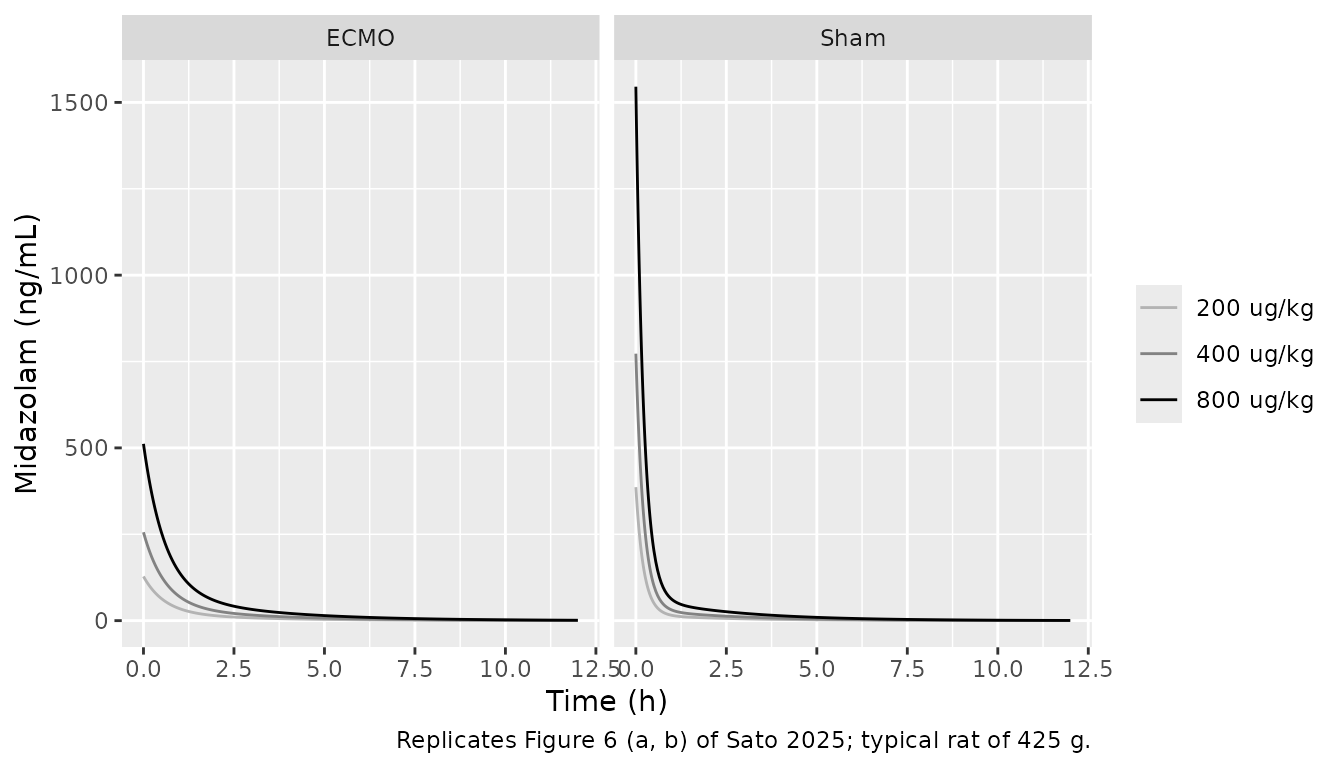
Figure 6 shows model-predicted profiles for three doses with and without ECMO over 0-12 h and 0-3 h. The typical-value curves below are for a 425 g rat (the middle of the 400-450 g range).
grid6 <- sort(unique(c(seq(0, 12, by = 0.05), seq(0, 0.5, by = 0.01))))
ev6 <- tidyr::expand_grid(
  dose_ugkg = c(200, 400, 800),
  ECMO_STATUS = c(0, 1)
) |>
  mutate(id = row_number(), amt = dose_ugkg * 0.425)
ev6 <- bind_rows(
  ev6 |> mutate(time = 0, evid = 1L, cmt = "central"),
  tidyr::expand_grid(ev6 |> select(-amt), time = grid6) |>
    mutate(amt = 0, evid = 0L, cmt = "central")
) |>
  arrange(id, time, desc(evid))

sim6 <- rxode2::rxSolve(
  rxode2::zeroRe(mod), events = ev6,
  keep = c("dose_ugkg"), rtol = 1e-10, atol = 1e-12
) |>
  as.data.frame() |>
  mutate(
    group = ifelse(ECMO_STATUS == 1, "ECMO", "Sham"),
    dose = factor(paste(dose_ugkg, "ug/kg"), levels = paste(c(200, 400, 800), "ug/kg"))
  )
#> ℹ parameter labels from comments will be replaced by 'label()'
#> ℹ omega/sigma items treated as zero: 'etalcl', 'etalvc'
#> Warning: multi-subject simulation without without 'omega'

ggplot(sim6, aes(time, Cc, colour = dose)) +
  geom_line() +
  facet_wrap(~group) +
  scale_colour_grey(start = 0.7, end = 0) +
  labs(
    x = "Time (h)", y = "Midazolam (ng/mL)", colour = NULL,
    caption = "Replicates Figure 6 (a, b) of Sato 2025; typical rat of 425 g."
  )
# Structural checks on the typical-value solve: initial concentration is
# dose / V1, the ECMO arm's is exactly 1/3.02 of the sham arm's, and the
# AUC to infinity equals dose / CL. These use the same parameters on both
# sides, so the tolerance is numerical only.
c0 <- sim6 |>
  filter(time == 0) |>
  select(dose_ugkg, group, Cc) |>
  tidyr::pivot_wider(names_from = group, values_from = Cc)
stopifnot(
  max(abs(c0$Sham / (c0$dose_ugkg * 0.425 / 0.22) - 1)) < 1e-6,
  max(abs(c0$ECMO / c0$Sham - 1 / 3.02)) < 1e-6
)
auc12 <- sim6 |>
  group_by(dose_ugkg, group) |>
  summarise(auc = sum(diff(time) * (head(Cc, -1) + tail(Cc, -1)) / 2), .groups = "drop")
# Trapezoidal AUC0-12h against dose/CL: the 1.7-h terminal half-life leaves
# ~1% of the AUC beyond 12 h and the 0.05-h grid adds ~1% trapezoid error.
stopifnot(max(abs(auc12$auc / (auc12$dose_ugkg * 0.425 / 0.69) - 1)) < 0.05)
knitr::kable(c0, digits = 0, caption = "Typical-value concentration at time 0 (ng/mL).")| dose_ugkg | Sham | ECMO |
|---|---|---|
| 200 | 386 | 128 |
| 400 | 773 | 256 |
| 800 | 1545 | 512 |
At 400 ug/kg the sham typical-value curve starts at about 773 ng/mL, matching the ~780 ng/mL read off Figure 6, and 800 ug/kg doubles it. The ECMO curves start 3.02-fold lower. The Figure 6 caption does not say which panel is which group; panel (b) starts lower, and the Results state that ECMO concentrations were lower immediately after the dose, so (b) is read as ECMO. Its initial concentrations are only about half of the sham ones (~390 vs ~780 ng/mL at 400 ug/kg), which does not follow from a 3.02-fold V1 effect; see Assumptions and deviations.
PKNCA validation
Table 2 of the paper reports a noncompartmental analysis of the observed data over 0-180 min. The same analysis is run here on the simulated rats, grouped by ECMO status.
sim_nca <- sim |>
  filter(!is.na(Cc)) |>
  select(id, time, Cc, group)
# The time-zero observation exists in every subject (the grid starts at 0);
# for an IV bolus it holds the post-dose concentration, which is correct.
stopifnot(all(tapply(sim_nca$time, sim_nca$id, min) == 0))

dose_df <- events |>
  filter(evid == 1) |>
  select(id, time, amt, group)

conc_obj <- PKNCA::PKNCAconc(sim_nca, Cc ~ time | group + id)
dose_obj <- PKNCA::PKNCAdose(dose_df, amt ~ time | group + id, route = "intravascular")
# AUC over the sampled 0-3 h window; half-life, CL and Vss from the same
# 0-3 h data extrapolated to infinity, as the paper's moment analysis does.
intervals <- data.frame(
  start = 0, end = c(3, Inf),
  auclast = c(TRUE, FALSE),
  half.life = c(FALSE, TRUE),
  cl.obs = c(FALSE, TRUE),
  vss.obs = c(FALSE, TRUE)
)
nca_res <- PKNCA::pk.nca(PKNCA::PKNCAdata(conc_obj, dose_obj, intervals = intervals))
Comparison against published NCA
Table 2 labels AUC0-180 min in ng/mL-hr, but its values (17,004 and 14,994) are 60 times what the Figure 3 means integrate to in ngh/mL (about 250 for the sham group); the column is in ngmin/mL. The reference AUCs below are the Table 2 values divided by 60. CL and Vss are in L and L/h because the dose is in ug and concentrations in ng/mL (ug/L).
published <- tibble::tribble(
  ~group, ~auclast, ~half.life, ~cl.obs, ~vss.obs,
  "ECMO", 17004.0 / 60, 7.4, 0.69, 1.21,
  "Sham", 14994.1 / 60, 0.88, 1.05, 0.92
)
cmp <- nlmixr2lib::ncaComparisonTable(
  simulated = nca_res,
  reference = published,
  by = "group",
  units = c(auclast = "ng*h/mL", half.life = "h", cl.obs = "L/h", vss.obs = "L"),
  tolerance_pct = 20
)
knitr::kable(cmp, caption = "Simulated (median) vs. published (mean, Table 2) NCA over 0-3 h. * differs from reference by >20%.")| NCA parameter | group | Reference | Simulated | % diff |
|---|---|---|---|---|
| AUClast (ng*h/mL) | ECMO | 283 | 207 | -27.0%* |
| AUClast (ng*h/mL) | Sham | 250 | 211 | -15.5% |
| t½ (h) | ECMO | 7.4 | 1.56 | -78.9%* |
| t½ (h) | Sham | 0.88 | 1.65 | +87.9%* |
| CL/F (L/h) | ECMO | 0.69 | 0.7 | +1.5% |
| CL/F (L/h) | Sham | 1.05 | 0.734 | -30.1%* |
| Vss/F (L) | ECMO | 1.21 | 1.06 | -12.7% |
| Vss/F (L) | Sham | 0.92 | 0.704 | -23.4%* |
The PKNCA helper labels clearance and Vss as CL/F and Vss/F; the dose is intravenous, so F = 1. Starred rows follow from the model structure and are not transcription errors:
- Clearance. The final model has one clearance (0.69 L/h) for both groups; ECMO was retained on V1 only. The simulated median clearance (about 0.7 L/h in both arms) matches the ECMO rats’ NCA clearance (0.69 L/h) and is below the sham rats’ (1.05 L/h), so the simulated ECMO AUC is also below the Table 2 value.
- Half-life. The paper’s ECMO half-life is 7.4 +/- 15.3 h over three rats, a spread that requires one rat with a half-life of more than a day; the sham value is 0.88 h. The model’s terminal half-life is 1.7 h in both groups, and a 0-3 h fit to the simulated rats gives about 1.6 h, between the two.
- Vss. The model’s typical Vss is V1 + V2 = 0.71 L (sham) and 1.15 L (ECMO), against 0.92 and 1.21 L by NCA.
# Structural gate: the sham-arm AUC0-3h is set by dose and CL and moves by
# tens of percent with a wrong dose basis (per kg vs absolute), unit or CL.
# Model typical value 220 ng*h/mL vs 250 from Table 2; the median over 200
# simulated rats is within about 15% of the typical value at any seed.
auc_sham <- as.data.frame(nca_res) |>
  filter(group == "Sham", PPTESTCD == "auclast")
stopifnot(abs(median(auc_sham$PPORRES) / (14994.1 / 60) - 1) < 0.35)
Assumptions and deviations
-
Covariate equation. The paper prints the ECMO model
as
theta_i = theta_pop * dic * exp(eta_i)withdicthe 0/1 ECMO indicator, which would set the parameter to zero in the sham rats. The model uses the conventional readingtheta_pop * 3.02^ECMO_STATUS, which reproduces the Discussion’s statement that V1 is 0.66 L with ECMO and 0.22 L without. - Parameter carrying the ECMO effect. One Results sentence reads “ECMO significantly influenced the CL of MDZ, and V1 was 3.02 times higher in the presence of ECMO”. Table 3 has a single ECMO coefficient, the Discussion assigns it to V1 (0.66 vs 0.22 L), and the reported typical CL has no ECMO-specific value, so the effect is placed on V1 only.
-
IIV scale. Table 3 reports IIV as CV%. The paper
does not say how CV% was computed from the NONMEM variance; the
conventional log-normal relation
omega^2 = log(CV^2 + 1)was used (0.617 for CL, 0.216 for V1). Read asomega = CV, the variances would be 0.854 and 0.241. - Timing of ECMO. Midazolam was given 2 min before ECMO started, and the first sample was taken before ECMO began. The paper’s covariate is per-rat, so the model applies the ECMO volume from the dose onward, as the paper did.
- Dose basis. The model’s parameters are absolute (L, L/h). The dose in the simulations is 400 ug/kg times a body weight drawn from 400-450 g, which reproduces the ~780 ng/mL initial concentration of the sham typical-value curve in Figure 6.
- Figure 6, ECMO panel. The published ECMO curves start at about half the sham concentration, not at 1/3.02 of it. The model is encoded from Table 3 and not adjusted to match the figure; the figure may show the mean of the Monte Carlo replicates, whose spread is not stated.
- Figure 3 means were read from the printed figure by the maintainers for the overlay only; no model value depends on them.
- No erratum or correction notice was found for this article (EuropePMC search, 2026-11-04).