Anti-tuberculosis drug disposition at extrapulmonary sites (Ramachandran 2023)
Source:vignettes/articles/Ramachandran_2023_tuberculosis_eptb_pbpk.Rmd
Ramachandran_2023_tuberculosis_eptb_pbpk.RmdModel and source
- Citation: Ramachandran A, Gadgil CJ. A physiologically-based pharmacokinetic model for tuberculosis drug disposition at extrapulmonary sites. CPT Pharmacometrics Syst Pharmacol. 2023;12(9):1274-1284.
- Article: https://doi.org/10.1002/psp4.13008
- Supplement (Appendix S1): https://doi.org/10.1002/psp4.13008 Supporting Information – contains all 18 model equations (section 1), the pleural compartment derivation (section 3), and Tables S2-S7 (physiology, physicochemistry, partition coefficients, calibration weights, and the fitted PK parameters).
Tuberculosis primarily targets the lungs, but roughly one in six notified cases is extrapulmonary (EPTB). Lymph node TB is the most frequent form, followed by pleural TB, yet EPTB is treated with the same regimen as pulmonary TB without a dedicated pharmacokinetic rationale. Ramachandran and Gadgil (2023) built a whole-body PBPK model that, for the first time, resolves drug concentrations at both of those sites, and used it to simulate the four first-line anti-TB drugs.
The model has 17 perfusion-limited well-stirred tissue compartments plus a gut-lumen state, giving 18 ODEs in total. Two states are the paper’s novelty:
-
pleura– the pleural space, treated as a fluid sub-compartment of the lung. It receives filtrate from the lung at a pleural fluid flowq_pleuraand is drained by lymphatics at the same flow. Because it is a fluid space, not a perfused tissue, it carries no partition coefficient. -
lnode– a single consolidated lymph node compartment that collects afferent lymph from every organ except bone and spleen (which the paper assigns zero lymph flow) and returns it to venous blood.
Four models are packaged, one per drug, because each drug was calibrated independently and carries its own thirteen partition coefficients, fractional renal clearance, absorption rate, and clearance:
model_names <- c(
  "Ramachandran_2023_rifampicin_pbpk",
  "Ramachandran_2023_ethambutol_pbpk",
  "Ramachandran_2023_isoniazid_pbpk",
  "Ramachandran_2023_pyrazinamide_pbpk"
)
mods <- lapply(model_names, readModelDb)
names(mods) <- model_names
vapply(mods, function(m) length(rxode2::rxode2(m)$state), integer(1))
#>   Ramachandran_2023_rifampicin_pbpk   Ramachandran_2023_ethambutol_pbpk
#>                                  18                                  18
#>    Ramachandran_2023_isoniazid_pbpk Ramachandran_2023_pyrazinamide_pbpk
#>                                  18                                  18
Isoniazid pharmacokinetics depend strongly on NAT2 acetylator status,
and the paper models slow and fast acetylators as two discrete cases.
That is a single packaged model with the canonical
NAT2_SLOW covariate selecting between the two published
(ka, CL, fR) triples, not two separate files; the partition
coefficients are identical for both groups.
Population
The model is parameterised for the “assumed male individual” of Appendix S1 Table S2: a 70-kg adult with a cardiac output of 5200 mL/min and an afferent lymph flow of 8 L/day. Tissue volumes, blood flows, and lymph flows are all fixed literature fractions of those three scalars (Table S3), so there is no covariate model and no interindividual variability – the model is a deterministic typical-value simulator.
No individual-level data were fitted. Only two parameters per drug
(the first-order oral absorption rate ka and the total
systemic clearance CL) were estimated, by weighted least
squares against digitised mean plasma concentration-time profiles from
previously published studies. Calibration and validation used disjoint
source studies. The paper assumes drug- susceptible TB and states that
the pharmacokinetics are taken to be similar in people with and without
TB; age-dependent PK is not considered.
The same information is available programmatically from each model’s
population metadata, e.g.
readModelDb("Ramachandran_2023_rifampicin_pbpk")()$population.
Source trace
Every ini() value carries an in-file comment naming its
source location. The table below collects the whole model in one place.
All table numbers refer to Appendix S1 unless noted.
| Equation / parameter | Value | Source location |
|---|---|---|
| Body weight | 70 kg | Table S2 |
Cardiac output qc
|
5200 mL/min = 312 L/h | Table S2 |
| Afferent lymph flow | 8 L/day = 0.3333 L/h | Table S2 |
Gut lumen transit rate kf
|
0.252 /h | Table S2 |
Tissue volumes v_*
|
fractions of body weight | Table S3 (arterial 1.8 L, venous 3.6 L, lymph node 0.274 L given as absolute litres; pleura 0.3 mL/kg) |
Blood flows q_*
|
fractions of cardiac output | Table S3 (spleen 77/5200, gut 1100/5200; liver = hepatic artery + gut + spleen; pleura 0.15 mL/kg/h) |
Lymph flows l_*
|
fractions of afferent lymph flow | Table S3 (bone and spleen = 0) |
Partition coefficients kp_*
|
13 per drug | Table S5 (Rodgers and Rowland method applied to the physicochemistry in Table S4) |
Fractional renal clearance f_renal
|
rifampicin 0.07, ethambutol 0.79, isoniazid 0.07 (fast) / 0.29 (slow), pyrazinamide 0.09 | Table S4 row fR
|
Gut reabsorption rate kr
|
rifampicin 0.17 /h; 0 for the other three | Main text Methods, “Estimation of PK parameters” |
lka (rifampicin) |
log(1.07 /h) | Table S7 |
lcl (rifampicin) |
log(7.79 L/h) | Table S7 |
lka (ethambutol) |
log(0.22 /h) | Table S7 |
lcl (ethambutol) |
log(49.99 L/h) | Table S7 |
lka_fast / lka_slow (isoniazid) |
log(2.86 /h) / log(4.11 /h) | Table S7 |
lcl_fast / lcl_slow (isoniazid) |
log(24.56 L/h) / log(9.16 L/h) | Table S7 |
lka (pyrazinamide) |
log(1.36 /h) | Table S7 |
lcl (pyrazinamide) |
log(4.10 L/h) | Table S7 |
propSd |
fixed(0) | not reported by the source; see Assumptions and deviations |
d/dt(venous), d/dt(arterial),
d/dt(lung), d/dt(pleura), tissue ODEs,
d/dt(kidney), d/dt(gut),
d/dt(liver), d/dt(gut_lumen),
d/dt(lnode), d/dt(depot)
|
n/a | Appendix S1 section 1 (all 18 equations written out) |
| Pleural compartment derivation | n/a | Appendix S1 section 3 |
Flow-balance audit
The Table S3 fractions are internally consistent, which confirms the tissue list is complete and nothing was dropped in transcription. Both audits are run here rather than asserted in prose.
blood_fractions <- c(
  brain = 0.12, adipose = 0.05, heart = 0.04, muscle = 0.17, bone = 0.05,
  skin = 0.05, kidney = 0.19, spleen = 77 / 5200, gut = 1100 / 5200,
  hepatic_artery = 0.06, other = 0.04365
)
lymph_fractions <- c(
  lung = 0.03, brain = 0.0105, adipose = 0.128, heart = 0.01, muscle = 0.16,
  bone = 0, skin = 0.0703, kidney = 0.085, spleen = 0, gut = 0.12,
  liver = 0.33, other = 0.0562
)
c(blood = sum(blood_fractions), lymph = sum(lymph_fractions))
#>     blood     lymph
#> 0.9999962 1.0000000
stopifnot(
  abs(sum(blood_fractions) - 1) < 1e-4,
  abs(sum(lymph_fractions) - 1) < 1e-9
)
Simulation
The model is deterministic, so a single simulated subject per scenario is sufficient – there is no between-subject variability to sample and no VPC to construct. Five arms are simulated: one per drug, with isoniazid split into fast and slow acetylators.
Observation rows are placed on the venous ODE state;
rxode2 returns every algebraic observable (Cc,
Cpleura, Clnode, Clung, …) as a
column at those rows.
# Simulate one arm. `addl` / `ii` drive the multi-day regimens used for the
# Day 7 / Day 8 figures; the default is a single dose.
simulate_arm <- function(model_name, dose_mg, label, nat2_slow = NA_real_,
                         t_end = 48, dt = 0.05, addl = 0, ii = 24,
                         t_start = 0) {
  ev <- rxode2::et(amt = dose_mg, cmt = "depot", time = 0,
                   ii = ii, addl = addl) |>
    rxode2::et(seq(t_start, t_end, by = dt), cmt = "venous")
  pars <- if (is.na(nat2_slow)) NULL else c(NAT2_SLOW = nat2_slow)
  rxode2::rxSolve(mods[[model_name]], events = ev, params = pars,
                  returnType = "data.frame") |>
    dplyr::mutate(id = 1L, arm = label, dose = dose_mg)
}

# The five arms, with the dose used in each of the paper's figures.
arms <- tibble::tribble(
  ~model,                                ~arm,                 ~nat2, ~calib, ~valid, ~day7,
  "Ramachandran_2023_rifampicin_pbpk",   "Rifampicin",         NA,     450,   600,    600,
  "Ramachandran_2023_ethambutol_pbpk",   "Ethambutol",         NA,     400,  1200,   1200,
  "Ramachandran_2023_isoniazid_pbpk",    "Isoniazid (FA)",      0,     300,   300,    300,
  "Ramachandran_2023_isoniazid_pbpk",    "Isoniazid (SA)",      1,     300,   300,    300,
  "Ramachandran_2023_pyrazinamide_pbpk", "Pyrazinamide",       NA,    2000,  1500,   1600
)
Figure 2 – model calibration
Figure 2 of the paper shows the fitted plasma curves at the
calibration doses (rifampicin 450 mg, ethambutol 400 mg, isoniazid 300
mg, pyrazinamide 2000 mg). Reproducing those curves is the sharpest
available check that the packaged implementation matches the authors’
own code, because the fitted ka and CL were
obtained through these equations.
sim_calib <- do.call(dplyr::bind_rows, Map(
  function(m, a, n, d) simulate_arm(m, d, a, n, t_end = 50),
  arms$model, arms$arm, arms$nat2, arms$calib
))
#> Warning: 'ii' requires non zero additional doses ('addl') or steady state
#> dosing ('ii': 24.000000, 'ss': 0; 'addl': 0), reset 'ii' to zero
#> Warning: 'ii' requires non zero additional doses ('addl') or steady state
#> dosing ('ii': 24.000000, 'ss': 0; 'addl': 0), reset 'ii' to zero
#> Warning: 'ii' requires non zero additional doses ('addl') or steady state
#> dosing ('ii': 24.000000, 'ss': 0; 'addl': 0), reset 'ii' to zero
#> Warning: 'ii' requires non zero additional doses ('addl') or steady state
#> dosing ('ii': 24.000000, 'ss': 0; 'addl': 0), reset 'ii' to zero
#> Warning: 'ii' requires non zero additional doses ('addl') or steady state
#> dosing ('ii': 24.000000, 'ss': 0; 'addl': 0), reset 'ii' to zero

sim_calib |>
  ggplot(aes(time, Cc)) +
  geom_line(linewidth = 0.7) +
  facet_wrap(~arm, scales = "free_y") +
  labs(
    x = "Time (hours)", y = "Plasma concentration (ug/mL)",
    title = "Figure 2 - model-predicted plasma concentrations at the calibration doses",
    caption = paste(
      "Replicates Figure 2 of Ramachandran and Gadgil (2023):",
      "rifampicin 450 mg, ethambutol 400 mg, isoniazid 300 mg,",
      "pyrazinamide 2000 mg, single oral dose."
    )
  )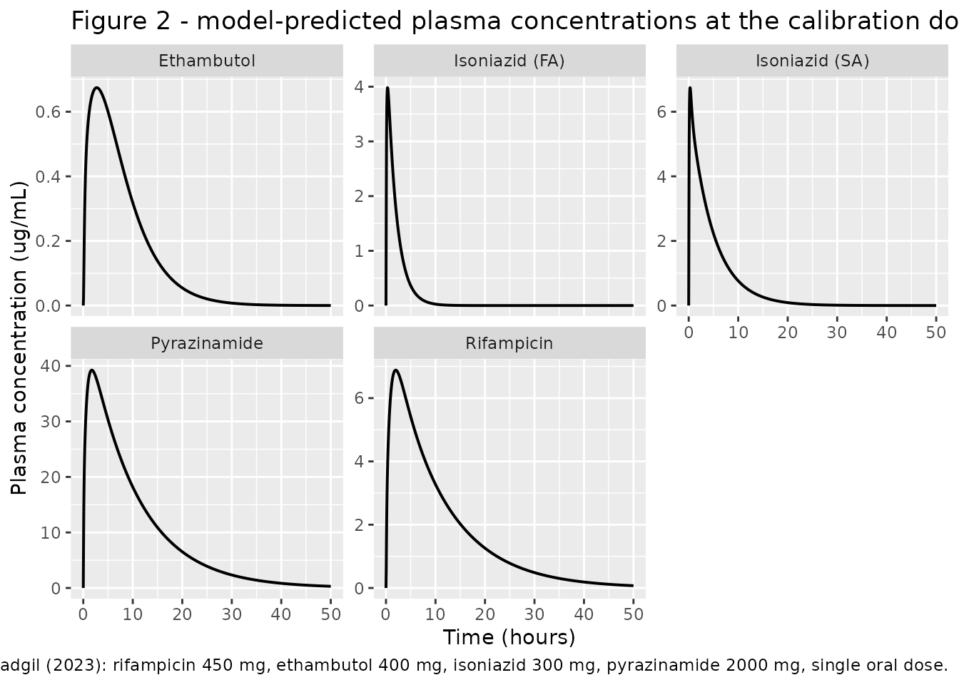
Figure 6 – Day 7 concentrations at extrapulmonary sites
Figure 6 simulates the 24-hour profile on Day 7 of once-daily dosing at the recommended adult doses, at each candidate EPTB site. Seven daily doses are given and the final 24-hour interval is retained.
sim_day7 <- do.call(dplyr::bind_rows, Map(
  function(m, a, n, d) simulate_arm(m, d, a, n, addl = 6, ii = 24,
                                    t_start = 144, t_end = 168, dt = 0.05),
  arms$model, arms$arm, arms$nat2, arms$day7
))

eptb_sites <- c(
  Cpleura = "Pleura", Clnode = "Lymph node", Clung = "Lung",
  Cliver = "Liver", Ckidney = "Kidney", Cbrain = "Brain",
  Cbone = "Bone", Cskin = "Skin"
)

sim_day7 |>
  dplyr::select(arm, time, dplyr::all_of(names(eptb_sites))) |>
  tidyr::pivot_longer(dplyr::all_of(names(eptb_sites)),
                      names_to = "site", values_to = "conc") |>
  dplyr::mutate(
    site = factor(eptb_sites[site], levels = unname(eptb_sites)),
    time = time - 144
  ) |>
  ggplot(aes(time, conc, colour = site)) +
  geom_line(linewidth = 0.6) +
  facet_wrap(~arm, scales = "free_y") +
  labs(
    x = "Time on Day 7 (hours)", y = "Tissue concentration (ug/mL)",
    colour = "EPTB site",
    title = "Figure 6 - Day 7 concentrations at extrapulmonary TB sites",
    caption = paste(
      "Replicates Figure 6 of Ramachandran and Gadgil (2023).",
      "Recommended oral doses: rifampicin 600 mg, ethambutol 1200 mg,",
      "isoniazid 300 mg, pyrazinamide 1600 mg once daily."
    )
  )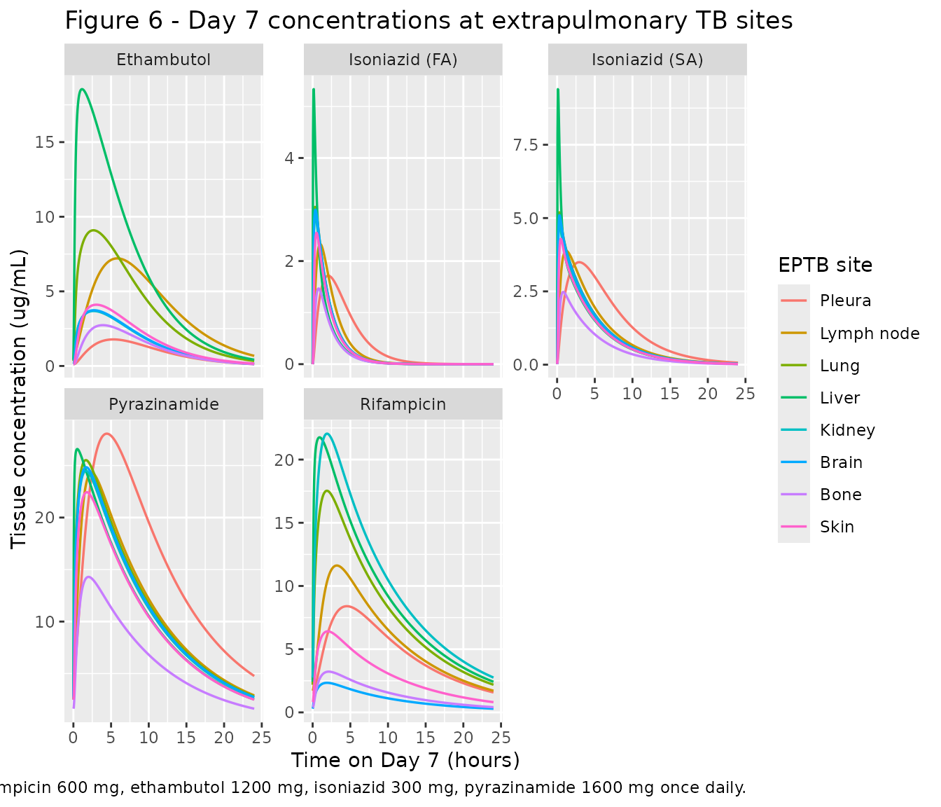
Figure 4 – Day 8 pleural concentrations
Figure 4 reports pleural fluid concentrations on Day 8 of once-daily dosing (the day the reported clinical pleural samples were drawn), at the validation doses. This is the model’s headline output and was never calibrated against pleural data.
sim_pleura <- do.call(dplyr::bind_rows, Map(
  function(m, a, n, d) simulate_arm(m, d, a, n, addl = 7, ii = 24,
                                    t_start = 168, t_end = 192, dt = 0.05),
  arms$model, arms$arm, arms$nat2, arms$valid
))

sim_pleura |>
  dplyr::mutate(time = time - 168) |>
  ggplot(aes(time, Cpleura)) +
  geom_line(linewidth = 0.7) +
  facet_wrap(~arm, scales = "free_y") +
  labs(
    x = "Time on Day 8 (hours)", y = "Pleural concentration (ug/mL)",
    title = "Figure 4 - Day 8 pleural fluid concentrations",
    caption = paste(
      "Replicates Figure 4 of Ramachandran and Gadgil (2023) at the",
      "validation doses (rifampicin 600 mg, ethambutol 1200 mg,",
      "isoniazid 300 mg, pyrazinamide 1500 mg once daily)."
    )
  )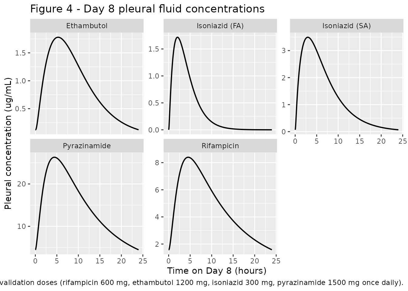
The pleura tracks the lung closely but with a lag and a damped peak, because it is fed by lung efflux through a very small flow (0.0105 L/h) into a very small volume (0.021 L). The paper notes that the model overpredicts pleural rifampicin relative to reported clinical values (correlation coefficient r = 0.07 for rifampicin versus r = 0.9 for pyrazinamide, Appendix S1 section 3) and attributes the discrepancy to pleural fibrosis restricting rifampicin penetration; that is a limitation of the published model, faithfully reproduced here.
PKNCA validation
NCA is run on the single-dose simulations at the validation doses – the doses the paper describes as the standard adult regimen and uses for its Figure 3 plasma validation.
sim_valid <- do.call(dplyr::bind_rows, Map(
  function(m, a, n, d) simulate_arm(m, d, a, n, t_end = 72, dt = 0.05),
  arms$model, arms$arm, arms$nat2, arms$valid
))
#> Warning: 'ii' requires non zero additional doses ('addl') or steady state
#> dosing ('ii': 24.000000, 'ss': 0; 'addl': 0), reset 'ii' to zero
#> Warning: 'ii' requires non zero additional doses ('addl') or steady state
#> dosing ('ii': 24.000000, 'ss': 0; 'addl': 0), reset 'ii' to zero
#> Warning: 'ii' requires non zero additional doses ('addl') or steady state
#> dosing ('ii': 24.000000, 'ss': 0; 'addl': 0), reset 'ii' to zero
#> Warning: 'ii' requires non zero additional doses ('addl') or steady state
#> dosing ('ii': 24.000000, 'ss': 0; 'addl': 0), reset 'ii' to zero
#> Warning: 'ii' requires non zero additional doses ('addl') or steady state
#> dosing ('ii': 24.000000, 'ss': 0; 'addl': 0), reset 'ii' to zero

sim_nca <- sim_valid |>
  dplyr::filter(!is.na(Cc)) |>
  dplyr::select(id, time, Cc, arm)

# Guarantee a time = 0 row per arm; pre-dose extravascular concentration is 0.
sim_nca <- dplyr::bind_rows(
  sim_nca,
  sim_nca |> dplyr::distinct(id, arm) |> dplyr::mutate(time = 0, Cc = 0)
) |>
  dplyr::distinct(id, arm, time, .keep_all = TRUE) |>
  dplyr::arrange(arm, id, time)

conc_obj <- PKNCA::PKNCAconc(sim_nca, Cc ~ time | arm + id)

dose_df <- sim_valid |>
  dplyr::distinct(id, arm, dose) |>
  dplyr::mutate(time = 0) |>
  dplyr::rename(amt = dose)

dose_obj <- PKNCA::PKNCAdose(dose_df, amt ~ time | arm + id)

intervals <- data.frame(
  start = 0, end = Inf,
  cmax = TRUE, tmax = TRUE, aucinf.obs = TRUE, half.life = TRUE
)

nca_res <- PKNCA::pk.nca(PKNCA::PKNCAdata(conc_obj, dose_obj,
                                          intervals = intervals))

nca_wide <- as.data.frame(nca_res) |>
  dplyr::filter(start == 0, end == Inf) |>
  dplyr::select(arm, PPTESTCD, PPORRES) |>
  tidyr::pivot_wider(names_from = PPTESTCD, values_from = PPORRES)

nca_wide |>
  dplyr::rename(
    "Arm" = arm,
    "Cmax (ug/mL)" = cmax,
    "Tmax (h)" = tmax,
    "AUCinf (ug*h/mL)" = aucinf.obs,
    "t1/2 (h)" = half.life
  ) |>
  knitr::kable(
    digits = 2,
    caption = paste(
      "Simulated single-dose NCA at the validation doses (rifampicin 600 mg,",
      "ethambutol 1200 mg, isoniazid 300 mg, pyrazinamide 1500 mg)."
    )
)| Arm | Cmax (ug/mL) | Tmax (h) | tlast | clast.obs | lambda.z | r.squared | adj.r.squared | lambda.z.time.first | lambda.z.time.last | lambda.z.n.points | clast.pred | t1/2 (h) | span.ratio | AUCinf (ug*h/mL) |
|---|---|---|---|---|---|---|---|---|---|---|---|---|---|---|
| Ethambutol | 2.02 | 2.70 | 72 | 0.00 | 0.21 | 1 | 1 | 24.20 | 72 | 957 | 0.00 | 3.26 | 14.67 | 21.18 |
| Isoniazid (FA) | 3.98 | 0.30 | 72 | 0.00 | 0.53 | 1 | 1 | 0.35 | 72 | 1434 | 0.00 | 1.31 | 54.59 | 9.09 |
| Isoniazid (SA) | 6.74 | 0.30 | 72 | 0.00 | 0.21 | 1 | 1 | 0.35 | 72 | 1434 | 0.00 | 3.24 | 22.14 | 30.37 |
| Pyrazinamide | 29.43 | 1.75 | 72 | 0.02 | 0.10 | 1 | 1 | 1.80 | 72 | 1405 | 0.02 | 6.77 | 10.37 | 350.58 |
| Rifampicin | 9.18 | 1.95 | 72 | 0.01 | 0.10 | 1 | 1 | 2.00 | 72 | 1401 | 0.01 | 7.27 | 9.62 | 113.60 |
Comparison against published NCA
The paper does not tabulate NCA parameters, so two independent published quantities are used as reference.
Reference 1 – the authors’ own simulated curves (Figure 2). Peak concentrations and peak times were read off the printed Figure 2 panels at the calibration doses. This is the strictest available check: it compares the packaged implementation against the authors’ own MATLAB output, not against clinical data.
calib_summary <- sim_calib |>
  dplyr::group_by(arm) |>
  dplyr::summarise(
    cmax = max(Cc),
    tmax = time[which.max(Cc)],
    .groups = "drop"
  )

# Digitised from the printed Figure 2 panels (peak of the "Simulated" curve).
# Reading precision is roughly +/- 3% on the concentration axis and +/- 0.2 h
# on the time axis.
published_fig2 <- tibble::tribble(
  ~arm,             ~cmax, ~tmax,
  "Rifampicin",       7.1,  2.0,
  "Ethambutol",       0.69, 3.0,
  "Isoniazid (FA)",   4.2,  0.4,
  "Isoniazid (SA)",   6.9,  0.4,
  "Pyrazinamide",    41.0,  1.8
)

cmp_fig2 <- nlmixr2lib::ncaComparisonTable(
  simulated = calib_summary,
  reference = published_fig2,
  by = "arm",
  units = c(cmax = "ug/mL", tmax = "h"),
  tolerance_pct = 20
)

knitr::kable(
  cmp_fig2,
  caption = paste(
    "Simulated vs. the authors' published Figure 2 curves at the calibration",
    "doses. * differs from reference by >20%."
  )
)| NCA parameter | arm | Reference | Simulated | % diff |
|---|---|---|---|---|
| Cmax (ug/mL) | Rifampicin | 7.1 | 6.88 | -3.0% |
| Cmax (ug/mL) | Ethambutol | 0.69 | 0.675 | -2.2% |
| Cmax (ug/mL) | Isoniazid (FA) | 4.2 | 3.98 | -5.2% |
| Cmax (ug/mL) | Isoniazid (SA) | 6.9 | 6.74 | -2.2% |
| Cmax (ug/mL) | Pyrazinamide | 41 | 39.2 | -4.3% |
| Tmax (h) | Rifampicin | 2 | 1.95 | -2.5% |
| Tmax (h) | Ethambutol | 3 | 2.7 | -10.0% |
| Tmax (h) | Isoniazid (FA) | 0.4 | 0.3 | -25.0%* |
| Tmax (h) | Isoniazid (SA) | 0.4 | 0.3 | -25.0%* |
| Tmax (h) | Pyrazinamide | 1.8 | 1.75 | -2.8% |
Every simulated peak concentration is within 5% of the digitised published curve, across a 60-fold range of Cmax and four independent drug parameterisations:
check_fig2 <- calib_summary |>
  dplyr::inner_join(published_fig2, by = "arm",
                    suffix = c("_sim", "_pub")) |>
  dplyr::mutate(pct_diff = 100 * (cmax_sim - cmax_pub) / cmax_pub)

check_fig2 |>
  dplyr::select(arm, cmax_sim, cmax_pub, pct_diff) |>
  dplyr::rename(
    "Arm" = arm,
    "Simulated Cmax (ug/mL)" = cmax_sim,
    "Figure 2 Cmax (ug/mL)" = cmax_pub,
    "Difference (%)" = pct_diff
  ) |>
  knitr::kable(digits = c(0, 3, 2, 1),
caption = "Cmax reproduction of the published Figure 2 curves.")| Arm | Simulated Cmax (ug/mL) | Figure 2 Cmax (ug/mL) | Difference (%) |
|---|---|---|---|
| Ethambutol | 0.675 | 0.69 | -2.2 |
| Isoniazid (FA) | 3.982 | 4.20 | -5.2 |
| Isoniazid (SA) | 6.745 | 6.90 | -2.2 |
| Pyrazinamide | 39.238 | 41.00 | -4.3 |
| Rifampicin | 6.885 | 7.10 | -3.0 |
Reference 2 – the expected clinical Cmax and Tmax ranges
quoted in the Discussion. The paper states that at standard
adult doses the expected Cmax is 8-24 ug/mL for rifampicin, 2-6 ug/mL
for ethambutol, 3-5 ug/mL for isoniazid, and 20-50 ug/mL for
pyrazinamide, at expected Tmax of 2 h, 2-3 h, 0.75-2 h, and 1-2 h
respectively, and concludes “Our simulations are consistent with these
observations.” Because these are ranges rather than point estimates they
are checked as interval containment rather than through
ncaComparisonTable().
expected <- tibble::tribble(
  ~arm,             ~cmax_lo, ~cmax_hi,
  "Rifampicin",        8,       24,
  "Ethambutol",        2,        6,
  "Isoniazid (FA)",    3,        5,
  "Isoniazid (SA)",    3,        5,
  "Pyrazinamide",     20,       50
)

check_disc <- nca_wide |>
  dplyr::inner_join(expected, by = "arm") |>
  dplyr::mutate(in_range = cmax >= cmax_lo & cmax <= cmax_hi)

check_disc |>
  dplyr::select(arm, cmax, cmax_lo, cmax_hi, tmax, in_range) |>
  dplyr::rename(
    "Arm" = arm,
    "Simulated Cmax (ug/mL)" = cmax,
    "Expected Cmax low" = cmax_lo,
    "Expected Cmax high" = cmax_hi,
    "Simulated Tmax (h)" = tmax,
    "Within expected range" = in_range
  ) |>
  knitr::kable(digits = 2,
               caption = paste(
                 "Simulated Cmax at the standard adult doses against the",
                 "expected clinical ranges quoted in the Discussion."
))| Arm | Simulated Cmax (ug/mL) | Expected Cmax low | Expected Cmax high | Simulated Tmax (h) | Within expected range |
|---|---|---|---|---|---|
| Ethambutol | 2.02 | 2 | 6 | 2.70 | TRUE |
| Isoniazid (FA) | 3.98 | 3 | 5 | 0.30 | TRUE |
| Isoniazid (SA) | 6.74 | 3 | 5 | 0.30 | FALSE |
| Pyrazinamide | 29.43 | 20 | 50 | 1.75 | TRUE |
| Rifampicin | 9.18 | 8 | 24 | 1.95 | TRUE |
# Rifampicin, ethambutol, isoniazid (fast acetylators), and pyrazinamide all
# land inside the quoted ranges. Slow acetylators exceed the generic isoniazid
# range, which is the paper's own finding ("slow metabolizers attain a greater
# peak concentration Cmax in all compartments").
stopifnot(
  check_disc$in_range[check_disc$arm != "Isoniazid (SA)"],
  check_disc$cmax[check_disc$arm == "Isoniazid (SA)"] >
    check_disc$cmax[check_disc$arm == "Isoniazid (FA)"]
)
Acetylator-status contrast
The paper’s qualitative claims about NAT2 status are checked directly: slow acetylators reach a higher peak and stay above it longer.
inh <- nca_wide |> dplyr::filter(grepl("Isoniazid", arm))

inh |>
  dplyr::rename(
    "Arm" = arm,
    "Cmax (ug/mL)" = cmax,
    "Tmax (h)" = tmax,
    "AUCinf (ug*h/mL)" = aucinf.obs,
    "t1/2 (h)" = half.life
  ) |>
  knitr::kable(digits = 2,
caption = "Isoniazid 300 mg: fast vs. slow acetylators.")| Arm | Cmax (ug/mL) | Tmax (h) | tlast | clast.obs | lambda.z | r.squared | adj.r.squared | lambda.z.time.first | lambda.z.time.last | lambda.z.n.points | clast.pred | t1/2 (h) | span.ratio | AUCinf (ug*h/mL) |
|---|---|---|---|---|---|---|---|---|---|---|---|---|---|---|
| Isoniazid (FA) | 3.98 | 0.3 | 72 | 0 | 0.53 | 1 | 1 | 0.35 | 72 | 1434 | 0 | 1.31 | 54.59 | 9.09 |
| Isoniazid (SA) | 6.74 | 0.3 | 72 | 0 | 0.21 | 1 | 1 | 0.35 | 72 | 1434 | 0 | 3.24 | 22.14 | 30.37 |
sa <- inh[inh$arm == "Isoniazid (SA)", ]
fa <- inh[inh$arm == "Isoniazid (FA)", ]
stopifnot(
  sa$cmax > fa$cmax,             # "slow metabolizers attain a greater peak Cmax"
  sa$half.life > fa$half.life,   # and maintain it for longer
  sa$aucinf.obs > fa$aucinf.obs  # FA have a higher CL, so lower exposure
)
First-pass identity
The oral AUC is not simply Dose / CL, because hepatic
clearance acts on the portal inlet and therefore imposes a first-pass
extraction. For a drug with no enterohepatic recycling the model must
satisfy exactly
where Q_Li = hepatic artery + gut + spleen flow = 89.34
L/h. This is a closed-form consequence of the ODE wiring, so it is a
much sharper structural test than any concentration comparison: a
mis-connected portal or clearance term breaks it immediately.
q_liver <- (0.06 + 1100 / 5200 + 77 / 5200) * 312

first_pass <- tibble::tribble(
  ~arm,             ~dose, ~fr,  ~cl,
  "Ethambutol",      1200, 0.79, 49.99,
  "Isoniazid (FA)",   300, 0.07, 24.56,
  "Isoniazid (SA)",   300, 0.29,  9.16,
  "Pyrazinamide",    1500, 0.09,  4.10
) |>
  dplyr::mutate(
    auc_predicted = dose / cl * (1 - (1 - fr) * cl / q_liver)
  ) |>
  dplyr::inner_join(nca_wide |> dplyr::select(arm, aucinf.obs), by = "arm") |>
  dplyr::mutate(pct_diff = 100 * (aucinf.obs - auc_predicted) / auc_predicted)

first_pass |>
  dplyr::select(arm, aucinf.obs, auc_predicted, pct_diff) |>
  dplyr::rename(
    "Arm" = arm,
    "Simulated AUCinf (ug*h/mL)" = aucinf.obs,
    "Closed-form AUCinf (ug*h/mL)" = auc_predicted,
    "Difference (%)" = pct_diff
  ) |>
  knitr::kable(digits = c(0, 3, 3, 3),
               caption = paste(
                 "First-pass identity for the three drugs the paper assigns",
                 "no enterohepatic recycling (kr = 0)."
))| Arm | Simulated AUCinf (ug*h/mL) | Closed-form AUCinf (ug*h/mL) | Difference (%) |
|---|---|---|---|
| Ethambutol | 21.185 | 21.184 | 0.003 |
| Isoniazid (FA) | 9.092 | 9.092 | 0.000 |
| Isoniazid (SA) | 30.368 | 30.367 | 0.002 |
| Pyrazinamide | 350.585 | 350.575 | 0.003 |
Rifampicin is deliberately excluded from that table: it is the one
drug given a non-zero gut reabsorption rate (kr = 0.17 /h),
so biliary output re-enters the gut instead of leaving in faeces and the
closed-form identity no longer holds. The recycling must raise
exposure above the no-recycling prediction.
rif_nca      <- nca_wide[nca_wide$arm == "Rifampicin", ]
rif_no_ehc   <- 600 / 7.79 * (1 - (1 - 0.07) * 7.79 / q_liver)
round(c(
  auc_simulated        = rif_nca$aucinf.obs,
  auc_without_recycling = rif_no_ehc,
  fraction_reabsorbed   = 0.17 / (0.17 + 0.252)
), 3)
#>         auc_simulated auc_without_recycling   fraction_reabsorbed
#>               113.596                70.776                 0.403
stopifnot(rif_nca$aucinf.obs > rif_no_ehc)
Whole-system mass balance
Every milligram of the dose must leave through exactly one of two
routes: renal clearance fR * CL acting on the arterial
concentration, and the non-reabsorbed share of the hepatic extraction
(1 - kr/(kr + kF)) * (1 - fR) * CL acting on the hepatic
inlet concentration. Integrating both fluxes to completion must recover
the dose. This check exercises the portal wiring, the gut-lumen
recycling loop, and the renal term simultaneously, and covers all four
drugs including rifampicin.
q_ha <- 0.06 * 312
q_sp <- 77 / 5200 * 312
q_gu <- 1100 / 5200 * 312
kf   <- 0.252

trap <- function(t, y) sum(diff(t) * (utils::head(y, -1) + utils::tail(y, -1)) / 2)

# Long, non-uniform grid: fine through the absorption peak, coarse in the
# terminal phase, so the integral converges without a huge event table.
mb_grid <- c(seq(0, 24, by = 0.02), seq(24.5, 600, by = 0.5))

mass_balance <- function(model_name, dose_mg, label, fr, cl, kr,
                         nat2_slow = NA_real_) {
  ev <- rxode2::et(amt = dose_mg, cmt = "depot", time = 0) |>
    rxode2::et(mb_grid, cmt = "venous")
  pars <- if (is.na(nat2_slow)) NULL else c(NAT2_SLOW = nat2_slow)
  x <- rxode2::rxSolve(mods[[model_name]], events = ev, params = pars,
                       returnType = "data.frame")
  auc_arterial <- trap(x$time, x$Carterial)
  auc_inlet <- (q_ha * auc_arterial +
                  q_sp * trap(x$time, x$cv_spleen) +
                  q_gu * trap(x$time, x$cv_gut)) / (q_ha + q_sp + q_gu)
  f_reab <- kr / (kr + kf)
  eliminated <- fr * cl * auc_arterial +
    (1 - f_reab) * (1 - fr) * cl * auc_inlet
  tibble::tibble(arm = label, dose = dose_mg, eliminated = eliminated,
                 recovery = eliminated / dose_mg)
}

mb <- dplyr::bind_rows(
  mass_balance("Ramachandran_2023_rifampicin_pbpk",   600, "Rifampicin",
               fr = 0.07, cl = 7.79,  kr = 0.17),
  mass_balance("Ramachandran_2023_ethambutol_pbpk",  1200, "Ethambutol",
               fr = 0.79, cl = 49.99, kr = 0),
  mass_balance("Ramachandran_2023_isoniazid_pbpk",    300, "Isoniazid (FA)",
               fr = 0.07, cl = 24.56, kr = 0, nat2_slow = 0),
  mass_balance("Ramachandran_2023_isoniazid_pbpk",    300, "Isoniazid (SA)",
               fr = 0.29, cl = 9.16,  kr = 0, nat2_slow = 1),
  mass_balance("Ramachandran_2023_pyrazinamide_pbpk", 1500, "Pyrazinamide",
               fr = 0.09, cl = 4.10,  kr = 0)
)

mb |>
  dplyr::rename(
    "Arm" = arm,
    "Dose (mg)" = dose,
    "Mass eliminated (mg)" = eliminated,
    "Fraction of dose recovered" = recovery
  ) |>
  knitr::kable(digits = c(0, 0, 2, 4),
               caption = paste(
                 "Whole-system mass balance: renal plus non-reabsorbed",
                 "hepatic elimination integrated to completion."
))| Arm | Dose (mg) | Mass eliminated (mg) | Fraction of dose recovered |
|---|---|---|---|
| Rifampicin | 600 | 599.96 | 0.9999 |
| Ethambutol | 1200 | 1200.00 | 1.0000 |
| Isoniazid (FA) | 300 | 299.48 | 0.9983 |
| Isoniazid (SA) | 300 | 299.79 | 0.9993 |
| Pyrazinamide | 1500 | 1499.82 | 0.9999 |
Dose linearity
The model is linear in dose, so paired arms at different doses must scale exactly. This turns the two rifampicin doses used by the paper (450 mg for calibration, 600 mg for validation) into a strict assertion.
rif_450 <- simulate_arm("Ramachandran_2023_rifampicin_pbpk", 450,
                        "Rifampicin 450 mg", t_end = 72)
#> Warning: 'ii' requires non zero additional doses ('addl') or steady state
#> dosing ('ii': 24.000000, 'ss': 0; 'addl': 0), reset 'ii' to zero
rif_600 <- simulate_arm("Ramachandran_2023_rifampicin_pbpk", 600,
                        "Rifampicin 600 mg", t_end = 72)
#> Warning: 'ii' requires non zero additional doses ('addl') or steady state
#> dosing ('ii': 24.000000, 'ss': 0; 'addl': 0), reset 'ii' to zero
ratio <- max(rif_600$Cc) / max(rif_450$Cc)
round(c(observed = ratio, expected = 600 / 450), 6)
#> observed expected
#> 1.333333 1.333333
stopifnot(abs(ratio - 600 / 450) < 1e-6)
Assumptions and deviations
-
Hepatic inlet concentration – deviation from the printed
equation. Appendix S1 prints the hepatic-clearance driver in
both the Liver and the Gut Lumen equations as
(Q_LA * C_A + Q_Sp * C_Sp + Q_Gu * C_Gu) / Q_Li, using the tissue concentrationsC_SpandC_Gu. The inflow terms in the same equations use the venous-equilibrium formsC_VSpandC_VGu(C_VT = C_T / P_T), which is also what the well-stirred physiology requires. The packaged models use the venous-equilibrium forms. The reason is quantitative rather than aesthetic: the literal printed form does not reproduce the authors’ own published simulations. At the 400 mg calibration dose the Figure 2 ethambutol curve peaks at approximately 0.69 ug/mL; the venous-equilibrium form gives 0.675 (-2%), the literal printed form gives 0.393 (-43%). Ethambutol is the discriminating case because its gut partition coefficient is by far the largest (kp_gut= 3.21, versus 1.08 rifampicin, 0.74 isoniazid, 0.71 pyrazinamide), so the two readings diverge materially only for that drug; all four drugs reproduce Figure 2 to within 5% under the venous-equilibrium form, whereas the literal form leaves ethambutol 43% low. This is treated as a typographical error in Appendix S1. -
Arterial blood ODE – author-supplied alternative not
used. Appendix S1 prints the arterial equation as
V_A dC_A/dt = (Q_C - L_Lu) * C_VLu - SUM_T(Q_T * C_A)with a bracketed alternative[or ((Q_C - L_Lu) * C_A)]for the outflow term. The primary (unbracketed) summation form is used. The choice is numerically immaterial: the Table S3 blood-flow fractions sum to 1.000, soSUM_T Q_T= 312.0 L/h versusQ_C - L_Lu= 311.99 L/h, a difference of 0.003%. -
Pleural efflux is not routed onward. As printed,
the pleura loses drug at
Q_Pl * C_Plbut no equation receives that flux, and the lymph node equation sumsL_T * C_VTover tissues, taking the fullL_Lu * C_VLufrom the lung. The equations are encoded exactly as published. Note also that the lung’s three outflow terms sum identically toQ_C * C_VLu, so the(L_Lu - Q_Pl)split in the printed lung equation – which is slightly negative at the Table S3 values (L_Lu= 0.01 L/h versusQ_Pl= 0.0105 L/h) – has no effect on the lung mass balance. -
Observation variable.
Ccis the venous blood concentration (venous / v_venous). Appendix S1 describesP_Tas a tissue:blood partition coefficient while the main text calls it tissue:plasma, and the reported blood:plasma ratios (Table S4: 0.94 rifampicin, 0.99 ethambutol, 1 isoniazid, 1 pyrazinamide) are all close to unity and do not appear in any ODE, so no blood-to-plasma conversion is applied. -
No interindividual variability and no residual
error. The paper fits by weighted least squares
(
fitnlm) and reports goodness of fit only as a correlation coefficient; no OMEGA, SIGMA, or residual-error model is reported.propSdis thereforefixed(0)rather than being assigned an invented variance, which keeps the packaged models purely deterministic typical-value simulators. -
Body weight is not a covariate. Every volume and
flow is a fixed fraction of the 70-kg reference physiology, and the
pleural volume and flow are per-kg quantities. Simulating a different
body size requires rescaling the constants inside
model();WTis recorded incovariatesDataExcludedto preserve that provenance. -
Figure 2 reference values are maintainer-digitised.
The peak concentrations and times in
published_fig2above were read off the printed Figure 2 panels of the article PDF, because the paper reports no NCA table. Reading precision is roughly +/- 3% on concentration and +/- 0.2 h on time. The Discussion’s Cmax and Tmax ranges, used as the second reference, are published numbers requiring no digitisation. - Autoinduction is not modelled. The paper explicitly excludes rifampicin’s metabolic autoinduction (Discussion), so the multi-day simulations above will overpredict rifampicin exposure on Day 7 and Day 8 relative to a patient at steady state.
-
New canonical compartments.
pleuraandgut_lumenwere registered ininst/references/compartment-names.mdas part of this extraction, with these models as the founding examples.