5-Fluorouracil colon-cancer QSP model (Ma 2022)
Source:vignettes/articles/Ma_2022_fluorouracil_qsp.Rmd
Ma_2022_fluorouracil_qsp.RmdModel and source
Ma, Almasan and Gurkan-Cavusoglu (2022) built an integrated mechanistic PK / PD model of 5-fluorouracil (5-FU) in colon cancer from three sub-models fitted in sequence by Bayesian MCMC to published mean data:
- a two-compartment plasma PK model with Michaelis-Menten elimination;
- a cellular model of 5-FU in tumour interstitial fluid, uptake into and efflux out of tumour cells, anabolism to fluoronucleotides, incorporation into RNA and DNA with delayed excision, FdUMP binding to thymidylate synthase (TS) in competition with dUMP, the resulting dNTP-pool imbalance with salvage feedback, and delayed DNA double-strand-break (DSB) induction;
- a tumour growth inhibition (TGI) model in which the anabolites slow logistic growth and the DSB excess over a drug-free baseline turns proliferating cells into damaged cells that die after a fixed life span.
The PK and cellular parameters (Table 1) are shared, and the TGI layer was re-estimated for each of nine xenograft datasets (Table 3 and Table 4). The library therefore carries nine model files, one per TGI model, each with the full shared PK and cellular layers.
models <- tibble::tribble(
  ~n, ~file,                                             ~cell,                 ~regimen,                                  ~mgkg, ~ii_day, ~ndose, ~dur_day, ~tv0,
  1L, "Ma_2022_fluorouracil_colon38_weekly_mouse_qsp",   "Colon 38",            "100 mg/kg weekly x 4",                    100,   7,       4L,     45,       125,
  2L, "Ma_2022_fluorouracil_colon26_daily_mouse_qsp",    "Colon 26",            "50 mg/kg daily x 4",                      50,    1,       4L,     7,        125,
  3L, "Ma_2022_fluorouracil_ht29_biw_mouse_qsp",         "HT29",                "20 mg/kg twice a week x 3 weeks",         20,    3.5,     6L,     21,       100,
  4L, "Ma_2022_fluorouracil_ht29_tiw_mouse_qsp",         "HT29",                "20 mg/kg three times a week x 3 weeks",   20,    7 / 3,   9L,     24,       100,
  5L, "Ma_2022_fluorouracil_sw620_daily_mouse_qsp",      "SW620",               "5 mg/kg daily x 9",                       5,     1,       9L,     9,        56.76,
  6L, "Ma_2022_fluorouracil_sw620_biw_mouse_qsp",        "SW620",               "20 mg/kg twice a week x 3 weeks",         20,    3.5,     6L,     26,       56.5,
  7L, "Ma_2022_fluorouracil_sw620_qod_mouse_qsp",        "SW620",               "20 mg/kg every other day x 2 weeks",      20,    2,       7L,     14,       71.3,
  8L, "Ma_2022_fluorouracil_ls174t_sensitive_mouse_qsp", "LS174T (sensitive)",  "50 mg/kg every other day x 6",            50,    2,       6L,     15,       125,
  9L, "Ma_2022_fluorouracil_ls174t_resistant_mouse_qsp", "LS174T (resistant)",  "50 mg/kg every other day x 6",            50,    2,       6L,     15,       125
)

# readModelDb() returns the model FUNCTION; rxode2::rxode() resolves it to
# the rxUi whose metadata and parameter values are readable.
ui <- lapply(setNames(models$file, models$n), \(f) rxode2::rxode(readModelDb(f)))- Citation: Ma C, Almasan A, Gurkan-Cavusoglu E. Computational analysis of 5-fluorouracil anti-tumor activity in colon cancer using a mechanistic pharmacokinetic/pharmacodynamic model. PLoS Comput Biol 2022;18(11):e1010685.
- Article: https://doi.org/10.1371/journal.pcbi.1010685
- Code and MCMC chains deposited by the authors: https://github.com/Chenhui88569/Computational-analysis-of-5-fluorouracil-anti-tumor-activity (Zenodo https://doi.org/10.5281/zenodo.7267874).
| TGI model | nlmixr2lib model | Cell line | Regimen | Initial tumour volume (mm^3) |
|---|---|---|---|---|
| 1 | Ma_2022_fluorouracil_colon38_weekly_mouse_qsp | Colon 38 | 100 mg/kg weekly x 4 | 125.00 |
| 2 | Ma_2022_fluorouracil_colon26_daily_mouse_qsp | Colon 26 | 50 mg/kg daily x 4 | 125.00 |
| 3 | Ma_2022_fluorouracil_ht29_biw_mouse_qsp | HT29 | 20 mg/kg twice a week x 3 weeks | 100.00 |
| 4 | Ma_2022_fluorouracil_ht29_tiw_mouse_qsp | HT29 | 20 mg/kg three times a week x 3 weeks | 100.00 |
| 5 | Ma_2022_fluorouracil_sw620_daily_mouse_qsp | SW620 | 5 mg/kg daily x 9 | 56.76 |
| 6 | Ma_2022_fluorouracil_sw620_biw_mouse_qsp | SW620 | 20 mg/kg twice a week x 3 weeks | 56.50 |
| 7 | Ma_2022_fluorouracil_sw620_qod_mouse_qsp | SW620 | 20 mg/kg every other day x 2 weeks | 71.30 |
| 8 | Ma_2022_fluorouracil_ls174t_sensitive_mouse_qsp | LS174T (sensitive) | 50 mg/kg every other day x 6 | 125.00 |
| 9 | Ma_2022_fluorouracil_ls174t_resistant_mouse_qsp | LS174T (resistant) | 50 mg/kg every other day x 6 | 125.00 |
Units and dosing
Time is in minutes throughout, as in the paper. The
plasma, interstitial and cellular states are concentrations, so a dose
is entered as the plasma concentration increment it produces. The
authors map 100 mg/kg to the first measured plasma concentration,
92.9936 ug/mL, and scale it linearly with dose (46.5 ug/mL at 50 mg/kg,
18.6 ug/mL at 20 mg/kg); this vignette uses
0.929936 * dose (mg/kg). The delay() terms
need a dense ODE solver and the interstitial-fluid exchange is fast (k03
= 136/min), so every solve below uses method = "dop853"
with a large maxsteps.
mgkg_to_conc <- function(mgkg) 0.929936306 * mgkg

# One treated or control animal on a regimen. Observation rows use the
# `anabolites` state as their compartment: it is one of the model's declared
# endpoints, and every other output is returned on the same rows.
sim_regimen <- function(file, mgkg, ii_day, ndose, tv0, times, params = NULL) {
  ev <- rxode2::et(times)
  if (mgkg > 0 && ndose > 1) {
    ev <- rxode2::et(
      amt = mgkg_to_conc(mgkg), cmt = "central",
      ii = ii_day * 1440, addl = ndose - 1
    ) |> rxode2::et(times)
  } else if (mgkg > 0) {
    ev <- rxode2::et(amt = mgkg_to_conc(mgkg), cmt = "central") |> rxode2::et(times)
  }
  ev <- as.data.frame(ev)
  ev$TUM_VOL <- tv0
  ev$cmt[ev$evid == 0] <- "anabolites"
  rxode2::rxSolve(
    readModelDb(file), ev,
    params = params, method = "dop853", maxsteps = 1e7,
    returnType = "data.frame"
  )
}
Population
There are no individual animals: every sub-model was fitted to group means taken from the literature (Ma 2022 Table 2 for the PK and cellular data, Table 3 for the tumour-volume data), so the model has no between-animal variability and every simulation below is deterministic.
- PK – C57BL/6 mice bearing Colon 38 tumours, 100 mg/kg intraperitoneal.
- Cellular layer – intracellular 5-FU and anabolites in C57BL/6 mice with C38 tumours (115 mg/kg); FU-RNA and FU-DNA in BALB/c mice with Colon 26-B tumours (80 mg/kg); TS-FdUMP complex and total TS in Wistar rats with dimethylhydrazine-induced colon carcinoma (100 mg/kg); dUMP in BALB/c mice with colon tumour 06/A (80 mg/kg); dNTP pools in L5178 lymphoma cells in vitro (1 uM); DSBs in OCI-AML2 leukaemia cells in vitro (3 umol/L).
- TGI layer – nine published xenograft or syngeneic colon-tumour datasets (Colon 38, Colon 26, HT29, SW620 and 5-FU-sensitive and -resistant LS174T), normalised to the starting tumour volume.
Source trace
| Quantity | Model variable / parameter | Source |
|---|---|---|
| Plasma PK (Eqs 1-3) |
central, peripheral1; lvmax,
lkm, lq, lvc,
lvp
|
Methods ‘PK model’; Table 1 ‘PK model’ |
| Interstitial 5-FU, uptake, efflux, anabolism (Eqs 4-6) |
isf, intracellular,
anabolites; q_isf, vmax_influx,
km_influx, vmax_efflux,
km_efflux, k03, vmax_anab,
km_anab
|
Eqs 4-6; Table 1 |
| FU-RNA, FU-DNA with delayed excision (Eqs 7-8) |
fu_rna, fu_dna; k65,
k56, k06, gamma_rna,
vmax_dna_in, km_dna_in,
vmax_dna_out, km_dna_out, k07,
gamma_dna, td_rna, td_dna
|
Eqs 7-8; Table 1 |
| TS-FdUMP complex, total TS, TS-dUMP, dUMP (Eqs 9-15) |
ts_fdump, dump; k95,
k59, k09, kd_dump,
g0_dump, kcat, k08,
alpha_ts, kd_ts, ts0
|
Eqs 9-15; Table 1 |
| dNTP-pool imbalance and salvage (Eqs 17-19) |
nucp, salvage; k1_dntp …
k10_dntp, kb_dntp, ka_dntp,
gamma_dntp
|
Eqs 17-19; Table 1 |
| DSB induction and drug-free baseline (Eqs 20-22) |
dsb, dsb_baseline; vmax_dntp,
km_dntp, vmax_hr, km_hr,
ki_hr, k0_dsb, gamma_dsb,
td_dsb
|
Eqs 20-22; Table 1; km_dntp from the deposited MCMC
chain |
| TGI (Eqs 23-28) |
cycling_cells, damaged_cells1,
tumor_vol; td_tv, ic50,
emax_damage, ec50_damage,
lambda_g, pmax, lambda_d,
gamma_tv
|
Eqs 23-28; Table 4 (per model) |
| Initial dUMP 3.878 and DSB 42.755 pmol/mg / thousand breaks |
dump(0), dsb(0),
dsb_baseline(0)
|
first (0 h) literature data points, as coded in the deposit |
| Initial tumour volume |
TUM_VOL covariate |
deposited code (CollectDataIntoNestedStructure.m) |
| Residual SDs (sqrt of the reported variances) |
addSd, addSd_<endpoint>
|
Table 1 and Table 4; PK and FU-RNA variances from the deposited MCMC chains |
| Dose-to-concentration mapping | 0.929936 * mg/kg |
deposited code |
Single 100 mg/kg dose: PK and cellular layers (Figures 2 and 3)
The PK and cellular parameters were fitted to a single intraperitoneal dose of 100 mg/kg (115 mg/kg and 80 mg/kg for some cellular data sets). The literature means the authors fitted are embedded in their deposited code and are overlaid here.
t_sd <- sort(unique(c(0, 2, 5, 10, 20, 30, 45, seq(60, 4320, by = 30))))
sd1 <- sim_regimen(models$file[1], 100, 7, 1L, 125, t_sd) |>
  mutate(pct_free_ts = 100 * ts_free / ts_total)

obs_sd <- dplyr::bind_rows(
  tibble::tibble(var = "Plasma 5-FU (ug/mL)", time = c(0, 10, 20, 30, 60, 90, 120, 240),
                 value = c(92.99, 70.25, 67.09, 48.33, 26.12, 11.39, 5.574, 1.753)),
  tibble::tibble(var = "Intracellular 5-FU (pmol/mg)", time = c(15, 30, 40, 50, 60, 70, 80, 90, 105, 120),
                 value = c(159.96, 133.32, 110.81, 39.86, 86.68, 62.38, 11.88, 46.23, 6.244, 8.477)),
  tibble::tibble(var = "Anabolites (pmol/mg)", time = c(15, 30, 40, 50, 60, 70, 80, 90, 105, 120),
                 value = c(29.34, 50.22, 42.82, 49.19, 43.57, 75.71, 67.86, 63.12, 73.78, 61.79)),
  tibble::tibble(var = "FU-RNA (pmol/mg)", time = c(2, 8, 24, 48, 72) * 60,
                 value = c(9.617, 6.488, 9.155, 2.366, 2.881) * 2),
  tibble::tibble(var = "FU-DNA (pmol/mg)", time = c(2, 8, 24, 48, 72) * 60,
                 value = c(15.53, 13.61, 15.76, 9.854, 14.43) * 2e-4),
  tibble::tibble(var = "TS-FdUMP complex (pmol/mg)", time = c(2, 6, 24, 32, 48) * 60,
                 value = c(0.0355, 0.0307, 0.0272, 0.0217, 0.0180)),
  tibble::tibble(var = "dUMP (pmol/mg)", time = c(3, 12, 24, 48) * 60,
                 value = c(5.770, 4.974, 5.552, 3.528)),
  tibble::tibble(var = "dNTP-pool imbalance", time = c(0.5, 1, 2, 4, 6, 8, 9, 12) * 60,
                 value = c(0.1532, 0.7109, 0.7337, 0.8817, 1.1337, 0.8240, 0.7070, 0.3747)),
  tibble::tibble(var = "DSB (thousands)", time = c(8, 24, 32, 48, 64, 72) * 60,
                 value = c(74.76, 74.28, 113.82, 226.81, 189.08, 132.25))
)

sim_sd <- sd1 |>
  transmute(
    time,
    "Plasma 5-FU (ug/mL)" = Cc,
    "Intracellular 5-FU (pmol/mg)" = intracellular,
    "Anabolites (pmol/mg)" = anabolites,
    "FU-RNA (pmol/mg)" = fu_rna,
    "FU-DNA (pmol/mg)" = fu_dna,
    "TS-FdUMP complex (pmol/mg)" = ts_fdump,
    "dUMP (pmol/mg)" = dump,
    "dNTP-pool imbalance" = nucp,
    "DSB (thousands)" = dsb
  ) |>
  pivot_longer(-time, names_to = "var")
ggplot(sim_sd, aes(time / 60, value)) +
  geom_line(colour = "firebrick") +
  geom_point(data = obs_sd, colour = "steelblue") +
  facet_wrap(~var, scales = "free_y", ncol = 3) +
  labs(x = "Time after dose (h)", y = NULL) +
  theme_bw()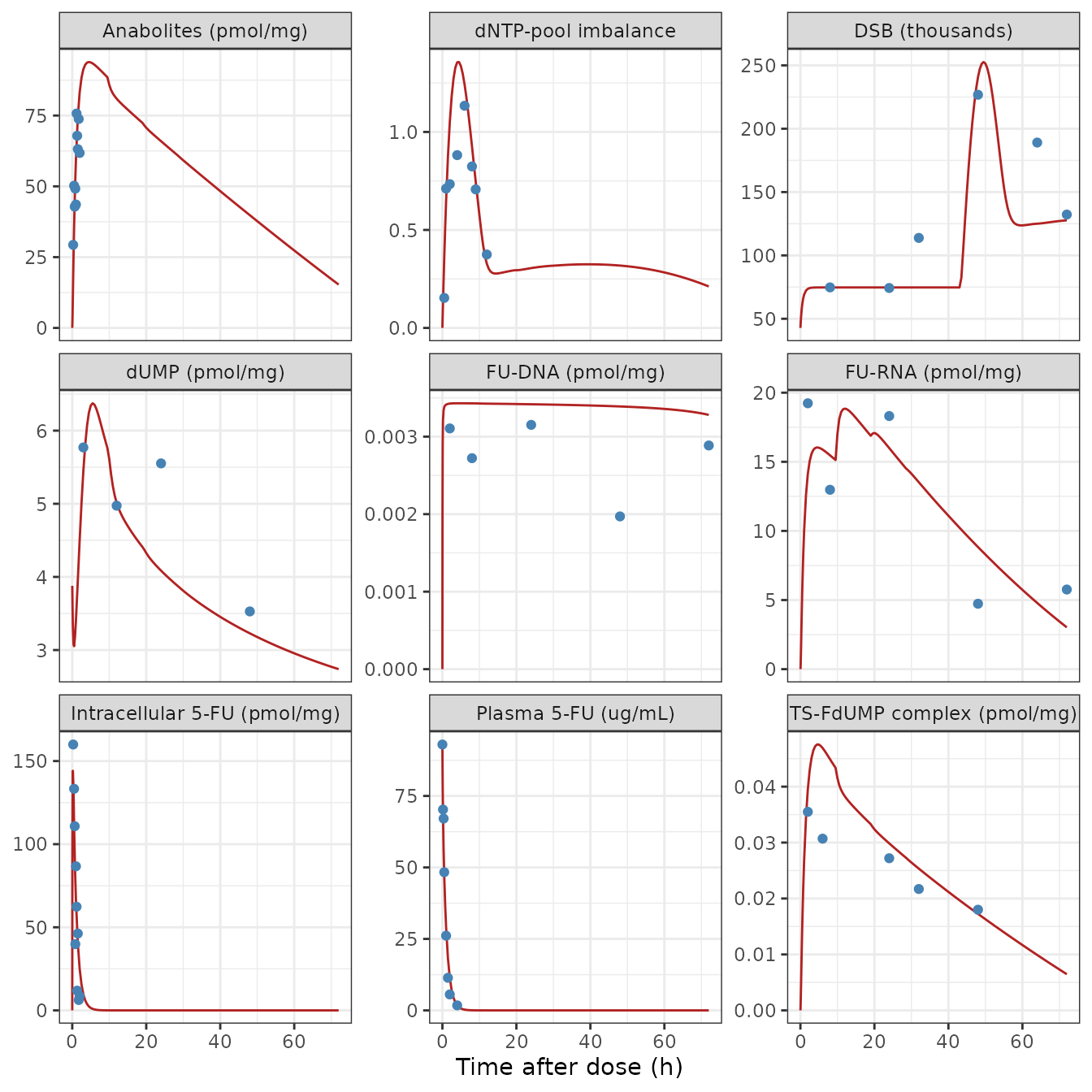
Replicates Figures 2 and 3 of Ma 2022: the shared PK and cellular layers after a single 100 mg/kg dose (line) against the literature means the authors fitted (points). The DSB data extend to 72 h, so the x-axis is cut at 3 days.
The free-TS fraction falls to its minimum about 5 h after the dose
and dUMP peaks at the same time, as described in the Results (‘Cellular
model’). The DSB count rises through the first hours toward the
drug-free baseline and only climbs above it after the 1.8-day delay
Td,DSB.
peak_dump_h <- sd1$time[which.max(sd1$dump)] / 60
min_free_h <- sd1$time[which.min(sd1$pct_free_ts)] / 60
stopifnot(
  abs(peak_dump_h - min_free_h) < 1.5,
  peak_dump_h > 3, peak_dump_h < 8
)
c(dUMP_peak_h = peak_dump_h, free_TS_minimum_h = min_free_h)
#>       dUMP_peak_h free_TS_minimum_h
#>               5.5               4.5
Plasma NCA
Ma 2022 reports no NCA for 5-FU. The table compares the PKNCA summary of the simulated plasma profile with that of the literature means the PK model was fitted to (Table 2, reference 65).
pk_sim <- sd1 |>
  filter(!is.na(Cc), time <= 240) |>
  transmute(id = 1L, treatment = "100 mg/kg", time, Cc)
pk_obs <- obs_sd |>
  filter(var == "Plasma 5-FU (ug/mL)") |>
  transmute(id = 1L, treatment = "100 mg/kg", time, Cc = value)
dose_df <- tibble::tibble(id = 1L, treatment = "100 mg/kg", time = 0, amt = mgkg_to_conc(100))

nca_fun <- function(conc_df) {
  conc <- PKNCAconc(conc_df, Cc ~ time | treatment + id)
  dose <- PKNCAdose(dose_df, amt ~ time | treatment + id)
  intervals <- data.frame(start = 0, end = 240, cmax = TRUE, auclast = TRUE, half.life = TRUE)
  pk.nca(PKNCAdata(conc, dose, intervals = intervals))
}
nca_sim <- nca_fun(pk_sim)
nca_obs <- nca_fun(pk_obs)
nlmixr2lib::ncaComparisonTable(nca_sim, nca_obs, by = "treatment",
  params = c("cmax", "auclast", "half.life"))
#>   NCA parameter treatment Reference Simulated % diff
#> 1          Cmax 100 mg/kg        93        93  +0.0%
#> 2       AUClast 100 mg/kg      4330      4800 +11.0%
#> 3            t½ 100 mg/kg      40.9        44  +7.4%
auc_ratio <- as.data.frame(nca_sim) |> filter(PPTESTCD == "auclast") |> pull(PPORRES) /
  (as.data.frame(nca_obs) |> filter(PPTESTCD == "auclast") |> pull(PPORRES))
stopifnot(abs(auc_ratio - 1) < 0.15)
auc_ratio
#> [1] 1.109559
Reproducing the authors’ multi-dose drivers
The authors pre-computed the anabolite and DSB time courses that
drive each TGI fit and deposited them with their code. Their multi-dose
simulation code enters the two excision delays Td,RNA and
Td,DNA in minutes (0.396 and 4.360 min),
whereas Table 1 reports them in days and their
single-dose fitting code converts days to minutes. The library models
carry the Table 1 values in days. Overriding the two delays with the
deposit’s minute values reproduces the deposited time courses, which
tests every other equation of the PK, cellular, dNTP and DSB layers
against the authors’ own numbers.
deposit_ref <- tibble::tribble(
  ~n, ~time,      ~a5,       ~dsb,
  1L, 62.0530,    58.415,    69.323,
  1L, 123.6431,   79.014,    73.709,
  1L, 278.9780,   87.803,    74.707,
  1L, 606.4480,   82.461,    74.724,
  1L, 1425.1276,  66.774,    74.724,
  1L, 2721.6811,  43.016,    164.59,
  1L, 4425.2147,  13.699,    127.96,
  1L, 7316.3939,  NA,        107.81,
  5L, 11629.6815, 3.0782,    90.682,
  8L, 1454.5650,  24.781,    74.724,
  8L, 3001.9917,  43.143,    166.46,
  8L, 14643.3688, 50.280,    145.58
)
deposit_lags <- c(td_rna = 0.39587 / 1440, td_dna = 4.35978 / 1440)

deposit_cmp <- deposit_ref |>
  group_by(n) |>
  group_modify(\(d, k) {
    m <- models[models$n == k$n, ]
    s <- sim_regimen(m$file, m$mgkg, m$ii_day, m$ndose, m$tv0,
      sort(unique(c(0, d$time))), params = deposit_lags)
    s <- s[match(d$time, s$time), ]
    mutate(d, a5_sim = s$anabolites, dsb_sim = s$dsb)
  }) |>
  ungroup() |>
  mutate(
    pct_a5 = 100 * (a5_sim - a5) / a5,
    pct_dsb = 100 * (dsb_sim - dsb) / dsb
  )

deposit_cmp |>
  mutate(across(c(a5_sim, dsb_sim, pct_a5, pct_dsb), \(x) signif(x, 4))) |>
  dplyr::rename(
    "TGI model" = n, "Time (min)" = time,
    "Anabolites, deposit" = a5, "Anabolites, model" = a5_sim, "Anabolites diff (%)" = pct_a5,
    "DSB, deposit" = dsb, "DSB, model" = dsb_sim, "DSB diff (%)" = pct_dsb
  ) |>
knitr::kable(caption = "Deposited anabolite and DSB time courses versus the library model with the deposit's minute-valued excision delays.")| TGI model | Time (min) | Anabolites, deposit | DSB, deposit | Anabolites, model | DSB, model | Anabolites diff (%) | DSB diff (%) |
|---|---|---|---|---|---|---|---|
| 1 | 62.0530 | 58.4150 | 69.323 | 58.420 | 69.32 | 0.004038 | -0.001427 |
| 1 | 123.6431 | 79.0140 | 73.709 | 79.040 | 73.71 | 0.036660 | 0.005562 |
| 1 | 278.9780 | 87.8030 | 74.707 | 87.850 | 74.70 | 0.058270 | -0.011430 |
| 1 | 606.4480 | 82.4610 | 74.724 | 82.540 | 74.71 | 0.093320 | -0.014330 |
| 1 | 1425.1276 | 66.7740 | 74.724 | 66.910 | 74.71 | 0.200500 | -0.014330 |
| 1 | 2721.6811 | 43.0160 | 164.590 | 43.200 | 164.20 | 0.422200 | -0.226700 |
| 1 | 4425.2147 | 13.6990 | 127.960 | 13.890 | 128.00 | 1.386000 | 0.042850 |
| 1 | 7316.3939 | NA | 107.810 | 0.000 | 107.80 | NA | 0.020330 |
| 5 | 11629.6815 | 3.0782 | 90.682 | 3.078 | 90.59 | -0.011060 | -0.097200 |
| 8 | 1454.5650 | 24.7810 | 74.724 | 24.830 | 74.71 | 0.211500 | -0.014330 |
| 8 | 3001.9917 | 43.1430 | 166.460 | 43.180 | 165.10 | 0.094620 | -0.813200 |
| 8 | 14643.3688 | 50.2800 | 145.580 | 50.430 | 145.00 | 0.300300 | -0.415300 |
Both sides are deterministic solves of the same equations, so the remaining differences are the rounding of the Table 1 values (printed to three or four significant figures) and solver error.
The two readings of the delays differ only in how long the excision of FU-RNA and FU-DNA runs at its pre-dose rate, so they diverge after a dose:
sd_dep <- sim_regimen(models$file[1], 100, 7, 1L, 125, t_sd, params = deposit_lags)
delay_units <- tibble::tibble(
  quantity = c("Peak anabolites (pmol/mg)", "Peak DSB (thousands)"),
  table1_days = c(max(sd1$anabolites), max(sd1$dsb)),
  deposit_minutes = c(max(sd_dep$anabolites), max(sd_dep$dsb))
) |>
  mutate(pct_diff = 100 * (table1_days - deposit_minutes) / deposit_minutes)
delay_units |>
  mutate(across(where(is.double), \(x) signif(x, 4))) |>
  dplyr::rename(
    Quantity = quantity, "Table 1 delays (days)" = table1_days,
    "Deposit delays (minutes)" = deposit_minutes, "Difference (%)" = pct_diff
  ) |>
knitr::kable(caption = "Single 100 mg/kg dose: effect of the excision-delay units.")| Quantity | Table 1 delays (days) | Deposit delays (minutes) | Difference (%) |
|---|---|---|---|
| Peak anabolites (pmol/mg) | 93.89 | 87.86 | 6.859 |
| Peak DSB (thousands) | 252.60 | 242.40 | 4.223 |
With the delays in days, the delayed-excision factor stays at its
pre-dose value for longer, so more fluoronucleotide returns from RNA to
the anabolite pool. The tumour-volume predictions are insensitive to
this because the anabolites act through A5^0.2 (the Table 5
comparison below shows the first-week exposure metrics agree to a few
per cent).
Tumour growth inhibition (Figure 4)
The literature tumour volumes (normalised to the first measurement) are the values the authors digitised into their deposit. TGI model 2 is simulated only through day 3: the published cellular layer becomes singular during the fourth daily 50 mg/kg dose (see ‘Assumptions and deviations’).
tgi_end_day <- ifelse(models$n == 2L, 3, models$dur_day)
tgi_ndose <- ifelse(models$n == 2L, 3L, models$ndose)

tgi_sim <- lapply(seq_len(nrow(models)), \(i) {
  m <- models[i, ]
  end_min <- tgi_end_day[i] * 1440
  obs_t <- tgi_obs$time_min[tgi_obs$model == m$n]
  times <- sort(unique(c(0, seq(0, 7 * 1440, by = 30), seq(0, end_min, by = 360),
    obs_t[obs_t <= end_min])))
  times <- times[times <= end_min]
  sim_regimen(m$file, m$mgkg, m$ii_day, tgi_ndose[i], m$tv0, times) |>
    mutate(n = m$n, rtv = tumor_vol / (m$tv0 / 1000))
}) |> bind_rows()

# The drug-free arm reduces to logistic growth with net rate lambda_g -
# lambda_d and ceiling Pmax * (1 - lambda_d / lambda_g); see the identity
# check below.
control_closed <- function(time, n, tv0) {
  th <- ui[[as.character(n)]]$theta
  p0 <- tv0 / 1000
  r <- th[["lambda_g"]] - th[["lambda_d"]]
  k <- th[["pmax"]] * (1 - th[["lambda_d"]] / th[["lambda_g"]])
  k / (1 + (k / p0 - 1) * exp(-r * time)) / p0
}
tgi_ctl <- models |>
  group_by(n) |>
  reframe(time = seq(0, dur_day * 1440, by = 360), rtv = control_closed(time, n, tv0))
short_reg <- c("100 mg/kg qw x4", "50 mg/kg qd x4", "20 mg/kg biw x3 wk", "20 mg/kg tiw x3 wk",
  "5 mg/kg qd x9", "20 mg/kg biw x3 wk", "20 mg/kg q2d x2 wk", "50 mg/kg q2d x6", "50 mg/kg q2d x6")
panel_lab <- setNames(paste0("(", models$n, ") ", models$cell, "\n", short_reg), models$n)
obs_long <- tgi_obs |>
  pivot_longer(c(rtv_treated, rtv_control), names_to = "arm", values_to = "rtv") |>
  filter(!is.na(rtv)) |>
  mutate(arm = ifelse(arm == "rtv_treated", "treated", "control"), n = model)
ggplot() +
  geom_line(data = tgi_sim, aes(time / 1440, rtv, colour = "treated")) +
  geom_line(data = tgi_ctl, aes(time / 1440, rtv, colour = "control"), linetype = 2) +
  geom_point(data = obs_long, aes(time_min / 1440, rtv, colour = arm, shape = arm)) +
  facet_wrap(~n, scales = "free", labeller = labeller(n = panel_lab)) +
  scale_colour_manual(values = c(treated = "steelblue", control = "firebrick")) +
  labs(x = "Time (days)", y = "Relative tumour volume", colour = NULL, shape = NULL) +
  theme_bw() +
  theme(legend.position = "bottom", strip.text = element_text(size = 7))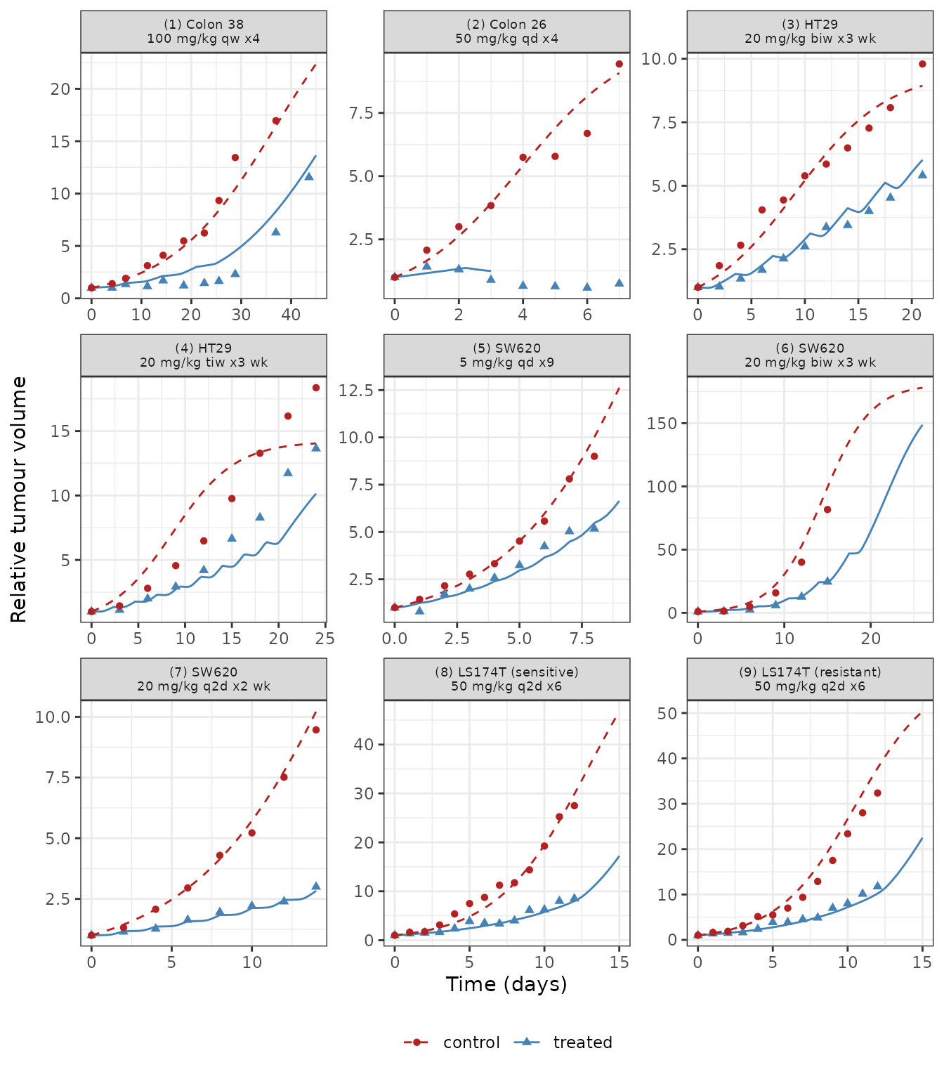
Replicates Figure 4 of Ma 2022: relative tumour volume of the treated (blue) and drug-free control (red) groups for the nine TGI models; points are the literature data the authors fitted.
tgi_fit <- tgi_obs |>
  rename(n = model) |>
  inner_join(tgi_sim |> select(n, time, rtv), by = c("n", "time_min" = "time")) |>
  group_by(n) |>
  summarise(
    n_obs = n(),
    median_abs_log_ratio = median(abs(log(rtv / rtv_treated))),
    final_sim = last(rtv), final_obs = last(rtv_treated)
  )
tgi_fit |>
  mutate(across(where(is.double), \(x) signif(x, 3))) |>
  dplyr::rename(
    "TGI model" = n, "Treated data points" = n_obs,
    "Median |log(sim/obs)|" = median_abs_log_ratio,
    "Final simulated" = final_sim, "Final observed" = final_obs
  ) |>
knitr::kable(caption = "Treated-group relative tumour volume, model versus literature data.")| TGI model | Treated data points | Median |log(sim/obs)| | Final simulated | Final observed |
|---|---|---|---|---|
| 1 | 11 | 0.2810 | 12.60 | 11.600 |
| 2 | 4 | 0.1080 | 1.25 | 0.891 |
| 3 | 11 | 0.1050 | 6.02 | 5.400 |
| 4 | 9 | 0.1750 | 10.10 | 13.600 |
| 5 | 9 | 0.0871 | 5.47 | 5.170 |
| 6 | 6 | 0.0879 | 24.60 | 24.500 |
| 7 | 8 | 0.0361 | 2.83 | 3.000 |
| 8 | 13 | 0.0787 | 8.00 | 8.500 |
| 9 | 13 | 0.1190 | 10.20 | 11.800 |
The treated-group fits match the quality shown in Figure 4, including the authors’ own remarks: model 4 (HT29, three times weekly), which reuses the model 3 efficacy parameters, fits only moderately, and model 1 over-predicts the Colon 38 tumours between weeks 2 and 6.
Drug-free arm identity
With no dose the anabolites and the DSB excess stay at zero, so Eq 23
reduces to dP/dt = lambda_g P (1 - P/Pmax) - lambda_d P
with a closed-form logistic solution. Solving the model for an untreated
TGI model 7 animal checks the TGI code path against it.
m7 <- models[models$n == 7L, ]
ctl7 <- sim_regimen(m7$file, 0, 1, 1L, m7$tv0, seq(0, m7$dur_day * 1440, by = 720)) |>
  mutate(closed = control_closed(time, 7L, m7$tv0), rtv = tumor_vol / (m7$tv0 / 1000))
stopifnot(
  max(abs(ctl7$rtv - ctl7$closed) / ctl7$closed) < 1e-4,
  all(ctl7$anabolites == 0), all(ctl7$damaged_cells1 == 0)
)
max(abs(ctl7$rtv - ctl7$closed) / ctl7$closed)
#> [1] 1.291755e-15
Exposure metrics over the first week (Table 5)
Table 5 integrates, over the first week of each regimen, the
anabolite amount (AUC_a), the relative DSB excess
(AUC_DSB) and the two effect functions Ea(t)
and EDSB(t) (AUC_e,a, AUC_e,DSB),
all with time in days. The authors’ values come from their minute-delay
drivers; the library values use the Table 1 delays in days. Model 2 is
omitted because its published driver is singular after day 3.
trapz <- function(x, y) sum(diff(x) * (head(y, -1) + tail(y, -1)) / 2)
table5 <- tibble::tribble(
  ~n, ~auc_ea, ~auc_edsb, ~auc_a,   ~auc_dsb,
  1L, 4.7900,  1.2874,    162.4190, 2.8343,
  3L, 4.9206,  0.3889,    17.2567,  0.9044,
  4L, 3.8823,  0.4494,    25.8850,  1.1920,
  5L, 5.0412,  1.7674,    4.2039,   0.6292,
  6L, 4.9206,  0.3895,    17.2567,  0.9044,
  7L, 3.1336,  0.4631,    34.5052,  1.3578,
  8L, 3.9429,  0.7832,    194.0453, 3.6296,
  9L, 3.8757,  2.4385,    194.0453, 3.6296
)
week <- tgi_sim |>
  filter(n %in% table5$n, time <= 7 * 1440) |>
  group_by(n) |>
  summarise(
    sim_auc_ea = trapz(time / 1440, e_a),
    sim_auc_edsb = trapz(time / 1440, e_dsb),
    sim_auc_a = trapz(time / 1440, anabolites),
    sim_auc_dsb = trapz(time / 1440, dsb_deviation)
  ) |>
  inner_join(table5, by = "n")
cmp5 <- week |>
  transmute(
    n,
    AUC_e_a = 100 * (sim_auc_ea - auc_ea) / auc_ea,
    AUC_e_DSB = 100 * (sim_auc_edsb - auc_edsb) / auc_edsb,
    AUC_a = 100 * (sim_auc_a - auc_a) / auc_a,
    AUC_DSB = 100 * (sim_auc_dsb - auc_dsb) / auc_dsb
  )
week |>
  transmute(
    n,
    "AUC_e,a (paper / model)" = paste(signif(auc_ea, 4), signif(sim_auc_ea, 4), sep = " / "),
    "AUC_e,DSB (paper / model)" = paste(signif(auc_edsb, 4), signif(sim_auc_edsb, 4), sep = " / "),
    "AUC_a (paper / model)" = paste(signif(auc_a, 4), signif(sim_auc_a, 4), sep = " / "),
    "AUC_DSB (paper / model)" = paste(signif(auc_dsb, 4), signif(sim_auc_dsb, 4), sep = " / ")
  ) |>
  dplyr::rename("TGI model" = n) |>
knitr::kable(caption = "Ma 2022 Table 5 versus the library models (first week, time in days).")| TGI model | AUC_e,a (paper / model) | AUC_e,DSB (paper / model) | AUC_a (paper / model) | AUC_DSB (paper / model) |
|---|---|---|---|---|
| 1 | 4.79 / 4.8 | 1.287 / 1.226 | 162.4 / 163.8 | 2.834 / 2.883 |
| 3 | 4.921 / 4.979 | 0.3889 / 0.3482 | 17.26 / 17.33 | 0.9044 / 0.9155 |
| 4 | 3.882 / 3.983 | 0.4494 / 0.3971 | 25.88 / 26 | 1.192 / 1.191 |
| 5 | 5.041 / 5.061 | 1.767 / 1.649 | 4.204 / 4.176 | 0.6292 / 0.6344 |
| 6 | 4.921 / 4.978 | 0.3895 / 0.3459 | 17.26 / 17.33 | 0.9044 / 0.9155 |
| 7 | 3.134 / 3.183 | 0.4631 / 0.4299 | 34.51 / 34.66 | 1.358 / 1.357 |
| 8 | 3.943 / 3.962 | 0.7832 / 0.7552 | 194 / 196.6 | 3.63 / 3.635 |
| 9 | 3.876 / 3.895 | 2.438 / 2.35 | 194 / 196.6 | 3.63 / 3.635 |
cmp5
#> # A tibble: 8 × 5
#>       n AUC_e_a AUC_e_DSB  AUC_a AUC_DSB
#>   <int>   <dbl>     <dbl>  <dbl>   <dbl>
#> 1     1   0.204     -4.76  0.836  1.71
#> 2     3   1.19     -10.5   0.442  1.23
#> 3     4   2.59     -11.6   0.442 -0.103
#> 4     5   0.390     -6.71 -0.669  0.827
#> 5     6   1.17     -11.2   0.442  1.23
#> 6     7   1.59      -7.17  0.446 -0.0367
#> 7     8   0.495     -3.58  1.29   0.140
#> 8     9   0.499     -3.63  1.29   0.140
stopifnot(
  max(abs(cmp5$AUC_a)) < 5,
  max(abs(cmp5$AUC_DSB)) < 5,
  max(abs(cmp5$AUC_e_a)) < 5,
  max(abs(cmp5$AUC_e_DSB)) < 20
)
The anabolite and DSB exposures agree within a few per cent despite
the different delay units. AUC_e,DSB runs 4-12% below Table
5 for a reason outside the model: the authors align their control DSB
curve to the treated time grid by interpolation, which leaves a relative
DSB excess of up to 1.3e-3 during the first 1.8 days, when the true
excess is exactly zero. EDSB raises that excess to the
power 0.2, so the artefact adds about 0.033 to every
AUC_e,DSB in Table 5 (recomputing Table 5 from the
deposited time courses reproduces the printed values, and the first 1.8
days contribute 0.0333 for both model 3 and model 8). Without it the
library values agree to within about 2%.
Assumptions and deviations
-
Excision delays in days. Table 1 lists
Td,RNA = 0.396andTd,DNA = 4.360in days, and the authors’ single-dose fitting code converts them from days to minutes; their multi-dose code (which generated the TGI drivers behind Table 4 and Figure 4) uses the same numbers as minutes. The library follows Table 1. The deposit’s behaviour is recovered withparams = c(td_rna = 0.39587 / 1440, td_dna = 4.35978 / 1440), as shown above; tumour-volume predictions differ by well under 1%. -
Values not printed in the paper.
K_dNTPappears in Eq 21 but not in Table 1, and the residual variances of plasma 5-FU and FU-RNA are not printed. All three are the posterior means of the authors’ deposited MCMC chains (Para_dNTP_DSB_col_2.mat,Para_PK_col.mat,Para_Cellular_col.mat) over the authors’ own burn-in, which reproduces every printed Table 1 value:K_dNTP = 151.918, plasma variance 52.112 (ug/mL)^2, FU-RNA variance 4.991 (pmol/mg)^2. The initial dUMP (3.878 pmol/mg) and DSB (42.755 thousand) levels and the initial tumour volumes of the nine datasets are also taken from the deposited code. -
Total TS resets at each dose. Eq 10 is a function
of
t; the authors restart the integration clock at every dose, sotis the time since the most recent dose (tad()). An undosed animal uses the time since the start of the simulation, as the authors’ control runs do. -
Model 2 is singular after its third dose. Under
daily 50 mg/kg the TS-FdUMP complex comes to exceed the total TS of Eq
10 after the fourth dose, so the free TS of Eq 11 turns negative. Once
it falls below
-K_dUMP * k08 / kcat(about -0.04 pmol/mg) the dUMP equation has a positive linear coefficient and grows exponentially toward the pole of Eq 13 atTSf = -K_dUMP; the solver stops shortly after 4500 min. The authors’ deposited model 2 driver is complex-valued over the same window. The model is encoded as published; only model 2’s regimen reaches this regime among the nine. -
Fractional powers guarded at zero.
(1 - TSf/TStotal)^gamma_dNTP,Nucp(t - Td,DSB)^gamma_DSB,A5^gamma_Tvand the relative DSB excess are evaluated onmax(x, 0). These quantities are non-negative in exact arithmetic; the guard only stops round-off below zero from producingNaN(the authors’ MATLAB code returns complex numbers there and keeps the real part). -
Doses as plasma-concentration increments. The PK
states are concentrations (Table 1 gives
Vmaxin ug/mL/min andKmin ug/mL), and the authors start each dose at the first measured plasma concentration (92.9936 ug/mL for 100 mg/kg), scaled linearly with dose. -
Units printed in Table 1.
k06andk07(min^-1 in Table 1) multiply an amount inside(1 + k * A)^gammaand therefore carry mg/pmol;k95multiplies TS and A5 and carries mg/pmol/min;G0is printed as mg/min but is a zero-order synthesis rate in pmol/mg/min; the dNTP-layer constants are printed as unitless althoughk1,k3,k5,k9andk10act as rates per minute. The parameter labels state the dimensionally consistent unit. -
Control and treated residual variances. Table 4
reports separate noise variances for the control and treated tumour
volumes. Both arms use the same equations, so the model exposes the
tumour volume twice:
tumor_vol(treated variance) andtumor_vol_control(control variance). -
Plasma PK with no drug loss to the tumour. Eq 4
adds
Q31 * Cpto the interstitial fluid without removing it from plasma, as published.