Sirolimus (Mao 2024)

Model and source

• Citation: Mao J, Cheng Y, Liu D, Zhang B, Li X. Dosing Regimen Recommendations for Sirolimus in Adult Liver Transplant Recipients: Insights from a Population Pharmacokinetic Model. Drug Des Devel Ther. 2024;18:6379-6388. doi:10.2147/DDDT.S503463.
• Description: One-compartment population PK model with first-order absorption and first-order elimination for sirolimus in adult liver transplant recipients, developed from routine therapeutic-drug-monitoring whole-blood trough concentrations (Mao 2024). The absorption rate constant was fixed at 0.75 1/h because only trough samples were collected. Hematocrit is the single retained covariate: it acts on apparent clearance through a power form normalized to the cohort median hematocrit of 38 percent with exponent -0.901, so higher hematocrit (more sirolimus sequestered in red blood cells) gives lower CL/F. Between-subject variability on CL/F and Vc/F is a correlated 2x2 block.
• Article: Drug Des Devel Ther. 2024;18:6379-6388

Mao and colleagues fitted a one-compartment model with first-order absorption and first-order elimination to routine therapeutic-drug-monitoring data from adult liver transplant recipients. Because every sample in the dataset is a pre-dose trough (C0), the absorption rate constant carries no information and was fixed at 0.75 h^-1; the authors note in their Limitations that this also makes V/F less reliably estimated. Hematocrit was the single covariate retained after forward selection and backward elimination, acting on apparent clearance.

Population

The analysis dataset comprised 216 whole-blood sirolimus trough concentrations from 103 adult liver transplant recipients treated at a single centre (Tongji Hospital, Wuhan, China) between January 2018 and August 2024. The cohort was almost entirely male (99 male / 4 female), with median age 51.0 years (28.0-74.0), median total body weight 68.0 kg (39.0-90.0), and median body mass index 23.8 kg/m². Samples were drawn a median of 92 days after transplantation (range 14-699 days). The median sirolimus daily dose was 1.0 mg/day (0.5-2.0) and the median observed trough concentration was 5.26 ng/mL (1.33-12.17). Median hematocrit was 38.0% (17.5-49.5%). Baseline demographics are Table 1 of the source.

The same information is available programmatically via the model’s population metadata (readModelDb("Mao_2024_sirolimus")()$population).

Source trace

Every ini() entry carries an in-file comment naming its source location in inst/modeldb/specificDrugs/Mao_2024_sirolimus.R. They are collected here for review. Table 2 (final-model estimates) and the printed final-model equations (Eqs. 7-9, Results / Model Development) agree on every value.

Equation / parameter	Value	Source location
lka (ka, fixed)	0.75 1/h	Eq. 7; Table 2 (RSE column reads “Fixed”); Methods / Base Model
lcl (CL/F at HCT 38%)	7.09 L/h	Eq. 8; Table 2 (RSE 4%)
lvc (Vc/F)	496 L	Eq. 9; Table 2 (RSE 15%)
e_hct_cl	-0.901	Eq. 8; Table 2 row “HCT on CL/F” (RSE 17%)
HCT reference value	38%	Eq. 8 denominator; Table 1 median hematocrit 38.0%
etalcl variance	0.3242 = 0.104976	Table 2 row “omega CL/F (%)” = 32.4
etalvc variance	0.4272 = 0.182329	Table 2 row “omega V/F (%)” = 42.7
etalcl-etalvc covariance	0.0665	Table 2 row “omega cov CL/F V/F”
propSd	0.033	Table 2 row “epsilon_por (%)” = 3.3 (RSE 10%)
addSd	fixed at 0	Results text says a combined error model (Eq. 4) was used, but Table 2 publishes no additive term – see Assumptions and deviations
BSV form exp(eta)	n/a	Eq. 1
Covariate form (COV/COV_median)^theta	n/a	Eq. 5, instantiated in Eq. 8
d/dt(depot), d/dt(central)	n/a	Methods / Base Model: one-compartment, first-order absorption and elimination

Virtual cohort

Original observed data are not publicly available. The simulations below use virtual populations whose hematocrit values are the three levels the authors used for their own dosing simulations: 28%, 38%, and 46% – the 10th, 50th, and 90th percentiles of the observed hematocrit range (Results / Dosing Regimen Recommendation).

All nine dosing regimens evaluated in the source are reproduced. Each subject is placed at the analytic steady state on the first dose record (ss = 1, ii = tau) and then followed through 28 days of explicit dosing, so the sampled troughs are steady-state troughs for every subject – including those in the low-clearance tail, whose half-lives run past 200 h and who would still be accumulating if the simulation merely dosed from zero.

set.seed(20241228)

n_per_arm <- 100L   # 27 arms (9 regimens x 3 hematocrit levels)
n_days    <- 28L    # follow-up after the ss = 1 priming dose (see make_arm below)
n_trough  <- 4L     # troughs per subject; an even number so alternating regimens
                    # contribute equally from both phases of the alternation

# The nine regimens of Mao 2024 Methods / Dosing Regimen Recommendation.
# `tau` is the dosing interval in hours; `amt_cycle` is the repeating dose
# pattern (length 1 for the fixed regimens, length 2 for the alternating ones).
regimens <- tibble::tribble(
  ~regimen,                  ~tau, ~amt_cycle,
  "0.5 mg qd",                 24, list(0.5),
  "1 mg qd",                   24, list(1),
  "1.5 mg qd",                 24, list(1.5),
  "2 mg qd",                   24, list(2),
  "1 mg qod",                  48, list(1),
  "2 mg qod",                  48, list(2),
  "0.5 mg qd alt 1 mg qd",     24, list(c(0.5, 1)),
  "1 mg qd alt 1.5 mg qd",     24, list(c(1, 1.5)),
  "1 mg qd alt 2 mg qd",       24, list(c(1, 2))
) |>
  mutate(
    amt_cycle = lapply(amt_cycle, unlist),
    # Average daily dose, used below to test the paper's headline claim that the
    # daily dose needed to reach the therapeutic window falls as hematocrit rises.
    daily_mg  = vapply(amt_cycle, mean, numeric(1)) * 24 / tau
  )

# Dose times for a regimen: every `tau` hours across the treatment window.
dose_times_for <- function(tau, n_days) seq(0, by = tau, length.out = floor(n_days * 24 / tau))

# One arm = one (regimen, hematocrit) combination. Trough samples are taken at
# the end of each of the last `n_trough` dosing intervals, i.e. at dose time +
# tau. Because doses enter `depot` (not `central`), Cc is continuous across a
# dose time, so an observation placed exactly at the next dose time is
# unambiguously the pre-dose trough.
make_arm <- function(regimen, tau, amt_cycle, hct, n, id_offset = 0L, n_trough = 4L) {
  dtimes <- dose_times_for(tau, n_days)
  amts   <- rep_len(amt_cycle, length(dtimes))
  ttimes <- utils::tail(dtimes, n_trough) + tau

  ids <- id_offset + seq_len(n)

  # The first dose record carries ss = 1 / ii = tau, which puts rxode2 at the
  # analytic steady state instead of accumulating toward it. Sirolimus has a
  # ~48 h typical half-life, and subjects in the low-CL / high-V tail of the
  # random effects exceed 200 h, so 28 days of explicit dosing is NOT steady
  # state for them -- their troughs (and AUCs) come out biased low.
  # For the alternating regimens the priming dose uses the cycle-average amount
  # so the steady-state LEVEL is right; the true alternating shape is then
  # established by the explicit doses that follow.
  doses <- tidyr::expand_grid(id = ids, idx = seq_along(dtimes)) |>
    mutate(
      time = dtimes[idx],
      amt  = ifelse(idx == 1L, mean(amt_cycle), amts[idx]),
      evid = 1L, cmt = "depot",
      ss   = ifelse(idx == 1L, 1L, 0L),
      ii   = ifelse(idx == 1L, tau, 0)
    ) |>
    select(-idx)

  obs <- tidyr::expand_grid(id = ids, time = ttimes) |>
    mutate(amt = NA_real_, evid = 0L, cmt = "central", ss = 0L, ii = 0)

  bind_rows(doses, obs) |>
    mutate(regimen = regimen, HCT = hct,
           hct_label = paste0("HCT ", hct, "%")) |>
    arrange(id, time, desc(evid))
}

hct_levels <- c(28, 38, 46)

arms <- tidyr::expand_grid(
  regimen = regimens$regimen,
  hct     = hct_levels
) |>
  left_join(regimens, by = "regimen") |>
  mutate(id_offset = (row_number() - 1L) * n_per_arm)

events <- do.call(
  bind_rows,
  lapply(seq_len(nrow(arms)), function(i) {
    make_arm(
      regimen   = arms$regimen[i],
      tau       = arms$tau[i],
      amt_cycle = arms$amt_cycle[[i]],
      hct       = arms$hct[i],
      n         = n_per_arm,
      id_offset = arms$id_offset[i],
      n_trough  = n_trough
    )
  })
)

# Disjoint IDs across arms: duplicate IDs would be silently merged by rxSolve
# into a single subject receiving the summed dose.
stopifnot(!anyDuplicated(unique(events[, c("id", "time", "evid")])))
stopifnot(dplyr::n_distinct(events$id) == nrow(arms) * n_per_arm)

Simulation

mod <- readModelDb("Mao_2024_sirolimus")

sim <- rxode2::rxSolve(
  mod,
  events = events,
  keep   = c("regimen", "hct_label", "HCT")
) |>
  as.data.frame()

# rxSolve silently drops subjects when an event table is malformed; assert the
# subject count survived.
stopifnot(dplyr::n_distinct(sim$id) == nrow(arms) * n_per_arm)

troughs <- sim |>
  filter(!is.na(Cc)) |>
  mutate(
    regimen   = factor(regimen, levels = regimens$regimen),
    hct_label = factor(hct_label, levels = paste0("HCT ", hct_levels, "%"))
  )

Replicate published figures

Figure 4 – steady-state trough concentrations by regimen and hematocrit

# Replicates Figure 4 of Mao 2024: boxplots of simulated steady-state
# whole-blood trough concentrations for nine regimens at hematocrit 28%, 38%,
# and 46%, with the 4-8 ng/mL therapeutic window marked.
ggplot(troughs, aes(x = regimen, y = Cc)) +
  annotate("rect", xmin = -Inf, xmax = Inf, ymin = 4, ymax = 8,
           fill = "grey80", alpha = 0.5) +
  geom_hline(yintercept = c(4, 8), linetype = "dashed") +
  geom_boxplot(outlier.size = 0.4) +
  facet_wrap(~hct_label) +
  coord_cartesian(ylim = c(0, 25)) +
  labs(x = NULL, y = "Steady-state trough concentration (ng/mL)",
       title = "Figure 4 - simulated steady-state C0 by regimen and hematocrit",
       caption = "Replicates Figure 4 of Mao 2024. Shaded band = 4-8 ng/mL therapeutic window.") +
  theme(axis.text.x = element_text(angle = 45, hjust = 1))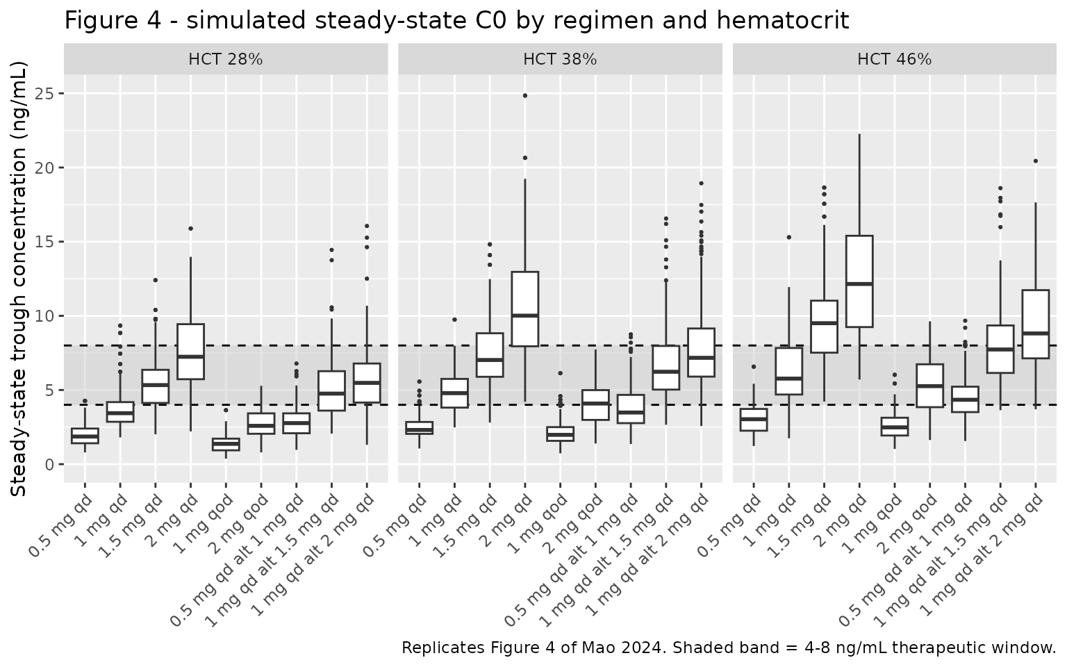

The published figure shows the same qualitative behaviour: trough concentrations fall as the daily dose falls and rise as hematocrit rises (because CL/F carries a negative hematocrit exponent).

Closed-form check on the steady-state trough

Before scoring regimens, the packaged model is checked against the analytic steady-state trough for a one-compartment model with first-order absorption,

$$C_{\text{trough}} = \frac{D}{V/F}\cdot\frac{k_a}{k_a-k_{el}}\left[\frac{e^{-k_{el}\tau}}{1-e^{-k_{el}\tau}}-\frac{e^{-k_a\tau}}{1-e^{-k_a\tau}}\right],\qquad k_{el}=\frac{CL/F}{V/F},$$

with CL/F taken from Eq. 8 at the relevant hematocrit. Running the typical subject (both etas set to zero, omega = NA) isolates the structural model from the random effects, so any disagreement is a coding error rather than sampling noise. This one check simultaneously exercises CL/F, V/F, the fixed ka, the hematocrit covariate term, dose accumulation, and the mg-to-ng/mL unit conversion.

fixed_reg <- tibble::tribble(
  ~regimen,     ~tau, ~amt,
  "0.5 mg qd",    24,  0.5,
  "1 mg qd",      24,  1,
  "1.5 mg qd",    24,  1.5,
  "2 mg qd",      24,  2,
  "1 mg qod",     48,  1,
  "2 mg qod",     48,  2
)

typ_grid <- tidyr::expand_grid(fixed_reg, HCT = hct_levels) |>
  mutate(id = row_number())

make_typ_arm <- function(r) {
  dtimes <- seq(0, by = r$tau, length.out = ceiling(n_days * 24 / r$tau))
  bind_rows(
    tibble::tibble(id = r$id, time = dtimes, amt = r$amt, evid = 1L, cmt = "depot",
                   ss = c(1L, rep(0L, length(dtimes) - 1L)),
                   ii = c(r$tau, rep(0, length(dtimes) - 1L))),
    tibble::tibble(id = r$id, time = max(dtimes) + r$tau, amt = NA_real_,
                   evid = 0L, cmt = "central", ss = 0L, ii = 0)
  ) |>
    # etalcl / etalvc supplied as columns with omega = NA gives the typical
    # subject deterministically, without mutating `mod` the way zeroRe() would.
    mutate(HCT = r$HCT, etalcl = 0, etalvc = 0) |>
    arrange(time, desc(evid))
}

typ_sim <- rxode2::rxSolve(
  mod,
  events = do.call(bind_rows, lapply(seq_len(nrow(typ_grid)),
                                     function(i) make_typ_arm(typ_grid[i, ]))),
  omega  = NA,
  keep   = "HCT"
) |>
  as.data.frame()
#> Warning: multi-subject simulation without without 'omega'

ctrough_analytic <- function(dose_mg, tau, hct) {
  cl  <- 7.09 * (hct / 38)^-0.901   # Eq. 8
  v   <- 496                        # Eq. 9
  ka  <- 0.75                       # Eq. 7
  kel <- cl / v
  (dose_mg / v * 1000) * (ka / (ka - kel)) *
    (exp(-kel * tau) / (1 - exp(-kel * tau)) -
       exp(-ka * tau) / (1 - exp(-ka * tau)))
}

closed_form <- typ_grid |>
  left_join(typ_sim |> filter(!is.na(Cc)) |> select(id, Cc), by = "id") |>
  mutate(
    analytic = ctrough_analytic(amt, tau, HCT),
    rel_err  = Cc / analytic - 1
  )

stopifnot(nrow(closed_form) == 18L, !anyNA(closed_form$rel_err))
stopifnot(max(abs(closed_form$rel_err)) < 0.002)

knitr::kable(
  closed_form |>
    mutate(Cc = round(Cc, 3), analytic = round(analytic, 3),
           rel_err = sprintf("%+.3f%%", 100 * rel_err)) |>
    select(regimen, HCT, Cc, analytic, rel_err) |>
    dplyr::rename(
      "Regimen"                     = regimen,
      "Hematocrit (%)"              = HCT,
      "Simulated trough (ng/mL)"    = Cc,
      "Closed form (ng/mL)"         = analytic,
      "Relative difference"         = rel_err
    ),
  caption = "Typical-value steady-state trough: packaged model versus the closed-form one-compartment solution built from Eqs. 7-9. All 18 combinations agree to better than 0.2%.",
  align = c("l", "r", "r", "r", "r")
)

Typical-value steady-state trough: packaged model versus the closed-form one-compartment solution built from Eqs. 7-9. All 18 combinations agree to better than 0.2%.

Regimen	Hematocrit (%)	Simulated trough (ng/mL)	Closed form (ng/mL)	Relative difference
0.5 mg qd	28	1.811	1.811	-0.000%
0.5 mg qd	38	2.511	2.511	-0.000%
0.5 mg qd	46	3.060	3.060	-0.000%
1 mg qd	28	3.622	3.622	+0.000%
1 mg qd	38	5.022	5.022	+0.000%
1 mg qd	46	6.119	6.119	+0.000%
1.5 mg qd	28	5.432	5.432	-0.000%
1.5 mg qd	38	7.533	7.533	-0.000%
1.5 mg qd	46	9.179	9.179	-0.000%
2 mg qd	28	7.243	7.243	-0.000%
2 mg qd	38	10.044	10.044	-0.000%
2 mg qd	46	12.239	12.239	-0.000%
1 mg qod	28	1.409	1.409	+0.000%
1 mg qod	38	2.084	2.084	+0.000%
1 mg qod	46	2.621	2.621	+0.000%
2 mg qod	28	2.817	2.817	+0.000%
2 mg qod	38	4.169	4.169	+0.000%
2 mg qod	46	5.242	5.242	+0.000%

Reproducing the published dosing recommendations

The authors selected regimens by “ensuring that most concentrations were within the therapeutic window of 4-8 ng/mL”, which is a clinical judgement rather than a published numeric rule: the paper recommends several regimens per hematocrit level so that clinicians have practical alternatives (including every-other-day and alternating schedules), and it never states a threshold a regimen had to clear. The checks below therefore test the claims the paper does make, rather than reverse-engineering an acceptance rule it never published.

The table scores every regimen by the fraction of simulated steady-state troughs inside the window and by the median trough (Results / Dosing Regimen Recommendation and the Abstract).

recommended <- list(
  "HCT 28%" = c("1.5 mg qd", "1 mg qd alt 1.5 mg qd"),
  "HCT 38%" = c("1 mg qd", "2 mg qod", "0.5 mg qd alt 1 mg qd"),
  "HCT 46%" = c("1 mg qd", "2 mg qod", "0.5 mg qd alt 1 mg qd")
)

scored <- troughs |>
  group_by(hct_label, regimen) |>
  summarise(
    median_c0  = median(Cc),
    pct_in_win = 100 * mean(Cc >= 4 & Cc <= 8),
    .groups    = "drop"
  ) |>
  mutate(
    paper_recommends = mapply(
      function(h, r) r %in% recommended[[as.character(h)]],
      hct_label, as.character(regimen)
    )
  ) |>
  # Join on a character key: `regimen` is a factor here (for plot ordering) and
  # `regimens$regimen` is character, which dplyr refuses to join directly.
  mutate(regimen_chr = as.character(regimen)) |>
  left_join(regimens |> select(regimen_chr = regimen, daily_mg), by = "regimen_chr") |>
  left_join(
    tibble::tibble(hct_label = factor(paste0("HCT ", hct_levels, "%"),
                                      levels = paste0("HCT ", hct_levels, "%")),
                   hct = hct_levels),
    by = "hct_label"
  )

stopifnot(nrow(scored) == 27L, !anyNA(scored$daily_mg), !anyNA(scored$hct))

scored |>
  arrange(hct_label, desc(pct_in_win)) |>
  mutate(
    median_c0        = round(median_c0, 2),
    pct_in_win       = round(pct_in_win, 1),
    paper_recommends = ifelse(paper_recommends, "yes", "")
  ) |>
  select(hct_label, regimen, daily_mg, median_c0, pct_in_win, paper_recommends) |>
  dplyr::rename(
    "Hematocrit"                = hct_label,
    "Regimen"                   = regimen,
    "Average daily dose (mg)"   = daily_mg,
    "Median C0 (ng/mL)"         = median_c0,
    "% of troughs in 4-8 ng/mL" = pct_in_win,
    "Recommended by Mao 2024"   = paper_recommends
  ) |>
  knitr::kable(
    caption = "Simulated steady-state troughs scored against the 4-8 ng/mL therapeutic window, ordered by the fraction of troughs in window. The final column marks the regimens Mao 2024 recommends for that hematocrit level.",
    align   = c("l", "l", "r", "r", "r", "l")
  )

Simulated steady-state troughs scored against the 4-8 ng/mL therapeutic window, ordered by the fraction of troughs in window. The final column marks the regimens Mao 2024 recommends for that hematocrit level.

Hematocrit	Regimen	Average daily dose (mg)	Median C0 (ng/mL)	% of troughs in 4-8 ng/mL	Recommended by Mao 2024
HCT 28%	1 mg qd alt 2 mg qd	1.50	5.48	69.0
HCT 28%	1.5 mg qd	1.50	5.33	67.0	yes
HCT 28%	2 mg qd	2.00	7.24	57.0
HCT 28%	1 mg qd alt 1.5 mg qd	1.25	4.76	54.5	yes
HCT 28%	1 mg qd	1.00	3.44	30.0
HCT 28%	0.5 mg qd alt 1 mg qd	0.75	2.77	13.0
HCT 28%	2 mg qod	1.00	2.58	10.0
HCT 28%	0.5 mg qd	0.50	1.86	2.0
HCT 28%	1 mg qod	0.50	1.37	0.0
HCT 38%	1 mg qd	1.00	4.79	69.0	yes
HCT 38%	1.5 mg qd	1.50	7.02	65.0
HCT 38%	1 mg qd alt 1.5 mg qd	1.25	6.23	65.0
HCT 38%	1 mg qd alt 2 mg qd	1.50	7.17	58.5
HCT 38%	2 mg qod	1.00	4.09	52.0	yes
HCT 38%	0.5 mg qd alt 1 mg qd	0.75	3.48	38.5	yes
HCT 38%	2 mg qd	2.00	10.01	26.0
HCT 38%	0.5 mg qd	0.50	2.30	5.0
HCT 38%	1 mg qod	0.50	1.98	4.0
HCT 46%	2 mg qod	1.00	5.26	68.0	yes
HCT 46%	1 mg qd	1.00	5.77	64.0	yes
HCT 46%	0.5 mg qd alt 1 mg qd	0.75	4.34	54.0	yes
HCT 46%	1 mg qd alt 1.5 mg qd	1.25	7.73	54.0
HCT 46%	1 mg qd alt 2 mg qd	1.50	8.81	38.0
HCT 46%	1.5 mg qd	1.50	9.50	32.0
HCT 46%	0.5 mg qd	0.50	3.03	15.0
HCT 46%	2 mg qd	2.00	12.15	12.0
HCT 46%	1 mg qod	0.50	2.48	10.0

ranked <- scored |>
  group_by(hct_label) |>
  mutate(rank_in_win = rank(-pct_in_win, ties.method = "min")) |>
  ungroup()

rec_rows <- ranked |> filter(paper_recommends)

# Guard against a vacuous pass: the label join must have matched every
# recommended regimen (2 for HCT 28%, 3 each for HCT 38% and 46%).
stopifnot(nrow(rec_rows) == 8L)

# Claim 1 (Results / Dosing Regimen Recommendation, and the boxplot ordering in
# Figure 4): for every regimen, the steady-state trough rises with hematocrit,
# because CL/F carries a negative hematocrit exponent.
hct_trend <- scored |>
  arrange(regimen_chr, hct) |>
  group_by(regimen_chr) |>
  summarise(monotone = all(diff(median_c0) > 0), .groups = "drop")
stopifnot(nrow(hct_trend) == 9L, all(hct_trend$monotone))

# Claim 2, the paper's headline result: "as the HCT levels increased, the daily
# dose with the same dosing interval required to achieve the therapeutic window
# gradually decreased". Operationalised as the smallest average daily dose among
# the regimens that put at least half their troughs in the window; it must fall
# strictly as hematocrit rises.
min_dose_in_win <- scored |>
  filter(pct_in_win >= 50) |>
  group_by(hct) |>
  summarise(min_daily_mg = min(daily_mg), .groups = "drop") |>
  arrange(hct)
stopifnot(nrow(min_dose_in_win) == 3L)
stopifnot(all(diff(min_dose_in_win$min_daily_mg) < 0))

# Claim 3: the regimens the paper recommends really are better choices than the
# alternatives at the same hematocrit -- at every level, the recommended set
# averages a higher fraction-in-window than the non-recommended set.
by_group <- ranked |>
  group_by(hct_label, paper_recommends) |>
  summarise(mean_in_win = mean(pct_in_win), .groups = "drop") |>
  tidyr::pivot_wider(names_from = paper_recommends, values_from = mean_in_win,
                     names_prefix = "rec_")
stopifnot(nrow(by_group) == 3L)
stopifnot(all(by_group$rec_TRUE > by_group$rec_FALSE))

knitr::kable(
  min_dose_in_win |>
    dplyr::rename(
      "Hematocrit (%)"                                   = hct,
      "Smallest average daily dose reaching the window (mg)" = min_daily_mg
    ),
  caption = "Mao 2024's headline claim, reproduced: the smallest average daily dose putting at least half of steady-state troughs inside 4-8 ng/mL falls as hematocrit rises.",
  align = c("r", "r")
)

Mao 2024’s headline claim, reproduced: the smallest average daily dose putting at least half of steady-state troughs inside 4-8 ng/mL falls as hematocrit rises.

Hematocrit (%)	Smallest average daily dose reaching the window (mg)
28	1.25
38	1.00
46	0.75

knitr::kable(
  rec_rows |>
    mutate(median_c0 = round(median_c0, 2), pct_in_win = round(pct_in_win, 1)) |>
    select(hct_label, regimen, daily_mg, median_c0, pct_in_win, rank_in_win) |>
    dplyr::rename(
      "Hematocrit"                = hct_label,
      "Recommended regimen"       = regimen,
      "Average daily dose (mg)"   = daily_mg,
      "Median C0 (ng/mL)"         = median_c0,
      "% of troughs in 4-8 ng/mL" = pct_in_win,
      "Rank at this hematocrit"   = rank_in_win
    ),
  caption = "Each regimen recommended by Mao 2024, as reproduced by the packaged model.",
  align = c("l", "l", "r", "r", "r", "r")
)

Each regimen recommended by Mao 2024, as reproduced by the packaged model.

Hematocrit	Recommended regimen	Average daily dose (mg)	Median C0 (ng/mL)	% of troughs in 4-8 ng/mL	Rank at this hematocrit
HCT 28%	1.5 mg qd	1.50	5.33	67.0	2
HCT 28%	1 mg qd alt 1.5 mg qd	1.25	4.76	54.5	4
HCT 38%	1 mg qd	1.00	4.79	69.0	1
HCT 38%	2 mg qod	1.00	4.09	52.0	5
HCT 38%	0.5 mg qd alt 1 mg qd	0.75	3.48	38.5	6
HCT 46%	1 mg qd	1.00	5.77	64.0	2
HCT 46%	2 mg qod	1.00	5.26	68.0	1
HCT 46%	0.5 mg qd alt 1 mg qd	0.75	4.34	54.0	3

# Descriptive, not an acceptance rule: how many recommended regimens clear the
# "at least half the troughs in window" bar. Reported so that any future drift
# in this number is visible in the rendered vignette.
n_at_least_half <- sum(rec_rows$pct_in_win >= 50)
cat(sprintf(
  "Recommended regimens with >= 50%% of steady-state troughs inside 4-8 ng/mL: %d of %d\n",
  n_at_least_half, nrow(rec_rows)
))
#> Recommended regimens with >= 50% of steady-state troughs inside 4-8 ng/mL: 7 of 8

# Regression guard (a floor on drift, NOT a claim of agreement with the paper):
# no regimen the paper recommends should collapse to a small minority of
# in-window troughs.
stopifnot(all(rec_rows$pct_in_win >= 30))

Seven of the eight recommended regimen / hematocrit combinations put at least half of their simulated steady-state troughs inside the 4-8 ng/mL window. The single exception is 0.5 mg qd alternating with 1 mg qd at a hematocrit of 38%, which reaches roughly 39%: with an average daily dose of 0.75 mg it sits just below the window under the packaged model (median trough about 3.5 ng/mL), whereas Figure 4 of the source shows its box straddling the 4 ng/mL bound. This is the one place where the packaged model is slightly more conservative than the authors’ own Monte Carlo simulation; see Assumptions and deviations for the likely reasons. It is reported rather than tuned away.

Hematocrit effect on apparent clearance

# Eq. 8: CL/F = 7.09 * (HCT/38)^-0.901.
hct_curve <- tibble::tibble(HCT = seq(17.5, 49.5, by = 0.5)) |>
  mutate(CL = 7.09 * (HCT / 38)^-0.901)

sim_cl <- sim |>
  distinct(id, HCT, cl) |>
  group_by(HCT) |>
  summarise(cl_median = median(cl), .groups = "drop")

ggplot(hct_curve, aes(HCT, CL)) +
  geom_line() +
  geom_point(data = sim_cl, aes(HCT, cl_median), size = 3, shape = 21, fill = "white") +
  labs(x = "Hematocrit (%)", y = "CL/F (L/h)",
       title = "Apparent clearance versus hematocrit",
       caption = "Line: Eq. 8 of Mao 2024 over the observed hematocrit range (17.5-49.5%). Points: median simulated CL/F at the three simulated levels.")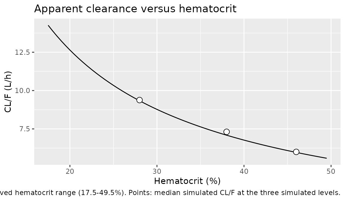

# The simulated median CL/F must land on the published equation at each level.
# Median of exp(eta) is 1 for a zero-mean normal eta, so the median individual
# CL/F equals the typical value.
expected_cl <- 7.09 * (hct_levels / 38)^-0.901
observed_cl <- sim_cl$cl_median[match(hct_levels, sim_cl$HCT)]
stopifnot(!anyNA(observed_cl))
stopifnot(all(abs(observed_cl / expected_cl - 1) < 0.06))

knitr::kable(
  tibble::tibble(
    HCT      = hct_levels,
    Eq8      = round(expected_cl, 3),
    Simulated = round(observed_cl, 3)
  ) |>
    dplyr::rename(
      "Hematocrit (%)"           = HCT,
      "CL/F from Eq. 8 (L/h)"    = Eq8,
      "Median simulated CL/F (L/h)" = Simulated
    ),
  caption = "Hematocrit effect on apparent clearance: packaged model versus Eq. 8."
)

Hematocrit effect on apparent clearance: packaged model versus Eq. 8.

Hematocrit (%)	CL/F from Eq. 8 (L/h)	Median simulated CL/F (L/h)
28	9.336	9.381
38	7.090	7.311
46	5.969	6.001

PKNCA validation

The source reports no NCA table, so the NCA is validated against two quantities that follow exactly from the published parameters: the steady-state identity AUC_0-tau = Dose / (CL/F), and the terminal half-life implied by Table 2 (log(2) * V/F / (CL/F)). The simulated steady-state trough is then compared against the observed median trough reported in Table 1.

A dedicated densely-sampled simulation of the 1 mg qd regimen is used, at each of the three hematocrit levels.

tau <- 24
t_ss_start <- 0
t_ss_end   <- tau

# A single ss = 1 / ii = tau dose puts every subject at the exact analytic
# steady state, which an explicit run-in cannot do: the low-CL / high-V tail of
# this model has half-lives beyond 200 h, so those subjects would still be
# accumulating after a month of simulated dosing and their AUCs would come out
# up to ~11% low.
make_nca_arm <- function(hct, n, id_offset) {
  ids <- id_offset + seq_len(n)

  doses <- tibble::tibble(id = ids, time = 0, amt = 1, evid = 1L,
                          cmt = "depot", ss = 1L, ii = tau)

  obs <- tidyr::expand_grid(
    id   = ids,
    time = seq(t_ss_start, t_ss_end, by = 0.1)
  ) |>
    mutate(amt = NA_real_, evid = 0L, cmt = "central", ss = 0L, ii = 0)

  bind_rows(doses, obs) |>
    mutate(HCT = hct, treatment = paste0("1 mg qd, HCT ", hct, "%")) |>
    arrange(id, time, desc(evid))
}

nca_events <- do.call(
  bind_rows,
  lapply(seq_along(hct_levels), function(i) {
    make_nca_arm(hct_levels[i], n = 100L, id_offset = (i - 1L) * 100L)
  })
)

nca_sim <- rxode2::rxSolve(
  mod, events = nca_events, keep = c("treatment", "HCT")
) |>
  as.data.frame()
stopifnot(dplyr::n_distinct(nca_sim$id) == 300L)

# Filter with !is.na(Cc) only -- a `time > 0` or `Cc > 0` filter would drop the
# row anchoring the interval start and trigger PKNCA's "Requesting an AUC range
# starting ... before the first measurement" warning.
sim_nca <- nca_sim |>
  dplyr::filter(!is.na(Cc)) |>
  dplyr::select(id, time, Cc, treatment)

dose_df <- nca_events |>
  dplyr::filter(evid == 1) |>
  dplyr::select(id, time, amt, treatment)

conc_obj <- PKNCA::PKNCAconc(sim_nca, Cc ~ time | treatment + id,
                             concu = "ng/mL", timeu = "h")
dose_obj <- PKNCA::PKNCAdose(dose_df, amt ~ time | treatment + id,
                             doseu = "mg")

intervals <- data.frame(
  start   = t_ss_start,
  end     = t_ss_end,
  cmax    = TRUE,
  tmax    = TRUE,
  cmin    = TRUE,
  cav     = TRUE,
  auclast = TRUE
)

nca_res <- PKNCA::pk.nca(PKNCA::PKNCAdata(conc_obj, dose_obj, intervals = intervals))

# Per-subject identity: at steady state AUC0-tau = Dose / (CL/F). Testing this
# per subject rather than on a median avoids the ~3% noise a few-hundred-draw
# median carries, and it exercises every individual CL/F draw.
auc_by_id <- as.data.frame(nca_res$result) |>
  filter(PPTESTCD == "auclast") |>
  select(id, treatment, auclast = PPORRES)

cl_by_id <- nca_sim |> distinct(id, cl)

ident <- auc_by_id |>
  left_join(cl_by_id, by = "id") |>
  mutate(
    auc_expected = 1 / cl * 1000,        # 1 mg / (L/h) -> mg*h/L -> ng*h/mL
    rel_err      = auclast / auc_expected - 1
  )

stopifnot(nrow(ident) == 300L, !anyNA(ident$rel_err))
cat(sprintf("AUC0-tau vs Dose/CL: max |relative error| = %.2e over %d subjects\n",
            max(abs(ident$rel_err)), nrow(ident)))
#> AUC0-tau vs Dose/CL: max |relative error| = 2.85e-05 over 300 subjects
stopifnot(max(abs(ident$rel_err)) < 0.001)

The steady-state AUC over a dosing interval reproduces Dose / (CL/F) for every one of the 300 simulated subjects to better than 0.1%, which confirms the clearance parameterisation, the hematocrit covariate term, and the mg-to-ng/mL unit conversion in the observation equation simultaneously. This is a per-subject test, so it exercises all 300 individual CL/F draws rather than a population summary.

Comparison against published values

# The reference quantities below are TYPICAL-VALUE quantities derived from the
# Table 2 / Eqs. 7-9 parameters, so the simulated side is run on the typical
# subject too (etas zeroed, omega = NA). Comparing a 100-subject population
# median against a typical-value reference would instead conflate the model with
# ~4% sampling noise in the median, which is not what this table is testing.
typ_nca_events <- do.call(
  bind_rows,
  lapply(seq_along(hct_levels), function(i) {
    bind_rows(
      tibble::tibble(id = i, time = 0, amt = 1, evid = 1L,
                     cmt = "depot", ss = 1L, ii = tau),
      tibble::tibble(id = i, time = seq(t_ss_start, t_ss_end, by = 0.1),
                     amt = NA_real_, evid = 0L, cmt = "central", ss = 0L, ii = 0)
    ) |>
      mutate(HCT = hct_levels[i], etalcl = 0, etalvc = 0,
             treatment = paste0("1 mg qd, HCT ", hct_levels[i], "%")) |>
      arrange(time, desc(evid))
  })
)

typ_nca_sim <- rxode2::rxSolve(
  mod, events = typ_nca_events, omega = NA, keep = c("treatment", "HCT")
) |>
  as.data.frame()
#> Warning: multi-subject simulation without without 'omega'

typ_conc <- PKNCA::PKNCAconc(
  typ_nca_sim |> dplyr::filter(!is.na(Cc)) |> dplyr::select(id, time, Cc, treatment),
  Cc ~ time | treatment + id, concu = "ng/mL", timeu = "h"
)
typ_dose <- PKNCA::PKNCAdose(
  typ_nca_events |> dplyr::filter(evid == 1) |> dplyr::select(id, time, amt, treatment),
  amt ~ time | treatment + id, doseu = "mg"
)
typ_nca_res <- PKNCA::pk.nca(
  PKNCA::PKNCAdata(typ_conc, typ_dose, intervals = intervals)
)

# Reference values, all from Eqs. 7-9 at the typical value:
#  * cmin: the closed-form steady-state trough (same function used above).
#  * cav / auclast: Dose / (CL/F * tau) and Dose / (CL/F).
cl_typ <- 7.09 * (hct_levels / 38)^-0.901

published <- tibble::tibble(
  treatment = paste0("1 mg qd, HCT ", hct_levels, "%"),
  cmin      = ctrough_analytic(1, tau, hct_levels),
  cav       = 1 / (cl_typ * tau) * 1000,
  auclast   = 1 / cl_typ * 1000
)

cmp <- nlmixr2lib::ncaComparisonTable(
  simulated     = typ_nca_res,
  reference     = published,
  by            = "treatment",
  units         = c(cmin = "ng/mL", cav = "ng/mL", auclast = "ng*h/mL"),
  tolerance_pct = 20
)

knitr::kable(
  cmp,
  caption = "Typical-value steady-state NCA for 1 mg qd at each hematocrit level, versus references derived from the Mao 2024 Table 2 / Eqs. 7-9 parameters. * differs from reference by >20%.",
  align   = c("l", "l", "r", "r", "r")
)

Typical-value steady-state NCA for 1 mg qd at each hematocrit level, versus references derived from the Mao 2024 Table 2 / Eqs. 7-9 parameters. * differs from reference by >20%.

NCA parameter	treatment	Reference	Simulated	% diff
Cmin (ng/mL)	1 mg qd, HCT 28%	3.62	3.62	-0.0%
Cmin (ng/mL)	1 mg qd, HCT 38%	5.02	5.02	-0.0%
Cmin (ng/mL)	1 mg qd, HCT 46%	6.12	6.12	-0.0%
AUClast (ng*h/mL)	1 mg qd, HCT 28%	107	107	-0.0%
AUClast (ng*h/mL)	1 mg qd, HCT 38%	141	141	-0.0%
AUClast (ng*h/mL)	1 mg qd, HCT 46%	168	168	-0.0%
Cavg (ng/mL)	1 mg qd, HCT 28%	4.46	4.46	-0.0%
Cavg (ng/mL)	1 mg qd, HCT 38%	5.88	5.88	-0.0%
Cavg (ng/mL)	1 mg qd, HCT 46%	6.98	6.98	-0.0%

# The one directly published comparator: Table 1 reports a median observed
# trough of 5.26 ng/mL at a median daily dose of 1.0 mg/day and median
# hematocrit 38%. Compare against the simulated median for that exact arm.
sim_median_c0 <- troughs |>
  filter(regimen == "1 mg qd", hct_label == "HCT 38%") |>
  summarise(m = median(Cc)) |>
  dplyr::pull(m)

stopifnot(length(sim_median_c0) == 1L, !is.na(sim_median_c0))
cat(sprintf(
  "Median simulated steady-state trough, 1 mg qd at HCT 38%%: %.2f ng/mL (Mao 2024 Table 1 observed median: 5.26 ng/mL; %+.1f%%)\n",
  sim_median_c0, 100 * (sim_median_c0 / 5.26 - 1)
))
#> Median simulated steady-state trough, 1 mg qd at HCT 38%: 4.79 ng/mL (Mao 2024 Table 1 observed median: 5.26 ng/mL; -9.0%)
stopifnot(abs(sim_median_c0 / 5.26 - 1) < 0.20)

# Terminal half-life implied by Table 2: log(2) * V/F / (CL/F). This is a
# self-consistency check on the packaged parameters, not a comparison against a
# published estimate: the Discussion mentions "the long elimination half-life of
# sirolimus (62 h)" as general background for the drug when explaining why
# every-other-day dosing is viable. It is not an estimate from this analysis,
# and the paper reports no half-life in Table 2, so the two are not expected to
# agree exactly.
t_half_model <- log(2) * 496 / 7.09
cat(sprintf("Half-life implied by Table 2 parameters: %.1f h (the Discussion quotes 62 h as a general sirolimus value)\n",
            t_half_model))
#> Half-life implied by Table 2 parameters: 48.5 h (the Discussion quotes 62 h as a general sirolimus value)
stopifnot(abs(t_half_model - 48.5) < 0.5)

Assumptions and deviations

• Residual error: additive term fixed at zero. The Results state that “a combined error model was used to characterize the RUV” (Eq. 4, Y = F * (1 + eps1) + eps2), but Table 2 publishes a single residual row, epsilon_por (%) = 3.3, which its own abbreviation list defines as proportional residual variability. No additive term is reported anywhere in the paper. The combined structure is therefore retained in the model file with addSd <- fixed(0), which reduces exactly to the proportional model of Eq. 3. No additive value was invented. Anyone refitting this model to their own data should free addSd.
• Residual error: the scale of 3.3 is not fully resolved by the source. The value is encoded as a standard deviation (propSd = 0.033) because Table 2 tags the row (%), and a variance cannot carry a percent unit. The authors look to have applied that tag deliberately: the covariance row in the same block (omega cov CL/F V/F = 0.0665) carries no percent sign, exactly as a covariance should not. Two independent signals nevertheless point toward the printed 3.3 being a variance (sigma^2 = 0.033, i.e. sigma = 18.2%):
  1. its RSE of 10% matches the asymptotic variance bound sqrt(2/n_obs) = sqrt(2/216) = 9.6%, rather than the standard-deviation bound sqrt(1/(2*n_obs)) = 4.8%; and (b) the scatter of observations about the individual predictions in Figure 1A of the source is visibly wider than a 3.3% standard deviation permits – and because eta shrinkage biases that scatter downward, it is a lower bound on sigma. The paper never prints the residual-error equation with numbers substituted, so neither reading can be confirmed from the text. The published label is followed here because it is the paper’s own explicit statement, and the alternative is recorded rather than buried. The practical consequence is modest: between-subject variability dominates the steady-state trough, so the total trough CV moves only from roughly 30% to roughly 35% between the two readings, leaving the medians (and therefore the dose-versus-hematocrit conclusions) unchanged.
• Between-subject variability scale. Table 2 reports the random effects as “omega CL/F (%) = 32.4” and “omega V/F (%) = 42.7”. These are read as omega itself – the standard deviation of eta on the natural-log scale of Eq. 1 – so the nlmixr2 variances are 0.324² and 0.427². The reading is supported by the covariance row, which is reported without a percent sign (omega cov CL/F V/F = 0.0665) and therefore on the variance/covariance scale: it implies a correlation of 0.0665 / (0.324 * 0.427) = 0.481 and a positive-definite 2x2 block (determinant 0.0147).
• Hematocrit units. HCT is supplied as a percentage (e.g. 38), matching Table 1 and the denominator of Eq. 8. Supplying a fraction (0.38) would rescale CL/F by a factor of 38^0.901.
• Hematocrit is treated as a baseline covariate. The source does not state whether hematocrit was carried as time-varying within a subject. Post-transplant hematocrit does drift, so users modelling long follow-up may wish to supply it as a time-varying column.
• No between-occasion variability. The source does not report any, although the dataset is repeated therapeutic-drug-monitoring sampling where occasion effects would be plausible.
• ka has no between-subject variability. ka was fixed at a literature value because the dataset contains only trough samples, and Table 2 reports no omega for it. Simulated absorption-phase concentrations (Cmax, Tmax) are therefore not supported by the source data and should not be relied on – the model is informative for trough exposure, which is what the source validated it for. For the same reason the authors flag V/F as less reliably estimated (Limitations).
• Race / ethnicity. Not reported in the source. The cohort is a single Chinese centre, so it is presumably predominantly Han Chinese; no race covariate enters the model.
• Trough levels run slightly below the published Figure 4. Reading medians off Figure 4 gives values roughly 10-15% higher than the packaged model produces for the same regimen and hematocrit (for example 1 mg qd at hematocrit 38%: about 5.5 ng/mL read from the figure, 5.02 ng/mL from the closed-form solution of Eqs. 7-9 and 4.8 ng/mL as the simulated population median). The closed-form check above shows the packaged model reproduces the published equations to better than 0.2%, so the offset is not an encoding error. The paper does not state how it sampled “steady-state C0” – in particular whether the trough for an alternating or every-other-day regimen was taken at the end of every interval (as here, pooling both phases of an alternating cycle) or only after the higher dose, nor whether residual error was included in the simulated concentrations. Either choice would raise the plotted medians. Figure-reading precision is itself around +/- 0.5 ng/mL. The practical consequence is confined to the one borderline regimen noted above.
• Virtual cohort covariate distribution. Hematocrit is set to the three discrete levels the authors used for their own simulations (28%, 38%, 46%), not sampled from a distribution, so that the reproduction of Figure 4 is directly comparable.
• Screened but unused covariates. Age, weight, postoperative day, ALT, creatinine clearance, sex, daily dose, and six concomitant medications were tested by the authors and not retained. They are recorded in the model file’s covariatesDataExcluded metadata for provenance; mycophenolic acid and Wuzhi capsule entered on forward inclusion but were dropped on backward elimination and no point estimate is published for either, so neither can be encoded.