Dapagliflozin (van der Walt 2013)
Source:vignettes/articles/vanderWalt_2013_dapagliflozin.Rmd
vanderWalt_2013_dapagliflozin.RmdModel and source
- Citation: van der Walt J-S, Hong Y, Zhang L, Pfister M, Boulton DW, Karlsson MO. A nonlinear mixed effects pharmacokinetic model for dapagliflozin and dapagliflozin 3O-glucuronide in renal or hepatic impairment. CPT Pharmacometrics Syst Pharmacol. 2013;2(5):e42. doi:10.1038/psp.2013.20.
- Description: see
mod$meta$description(full text printed in the source-trace section above). - Article: https://doi.org/10.1038/psp.2013.20 (open-access, CC BY-NC-ND).
Population
The model was built on pooled data from three Bristol-Myers Squibb clinical studies in 227 subjects:
- Study MB102007 (NCT00554450) – 40 adults: 8 healthy volunteers and 32 patients with type 2 diabetes mellitus (DIS_DIAB) spanning normal to severe renal impairment. A 50-mg single dose of oral dapagliflozin was followed by 20-mg q.d. for 7 days.
- Study MB102027 – 24 adults in a 5-day single-dose 10-mg hepatic- impairment substudy: 18 patients with hepatic impairment (Child-Pugh Class A mild = 6, Class B moderate = 6, Class C severe = 6) plus 6 age-, weight-, gender-, and smoking-status-matched healthy controls.
- Study MB102029 (NCT00663260) – a 52-week phase 3 trial in 163 DIS_DIAB subjects with moderate renal impairment, receiving 10-mg daily oral dapagliflozin.
Pooled demographics: weight range 51.8-148.3 kg, age range 25-92 years (per-study medians 63 / 43 / 67 years), 32.6% female, baseline creatinine clearance (IBW-corrected Cockcroft-Gault) range 13-143 mL/min. See van der Walt 2013 Table 2.
The same information is available programmatically as
readModelDb("vanderWalt_2013_dapagliflozin")$population.
Source trace
The per-parameter origin is recorded as an in-file comment next to
each ini() entry in
inst/modeldb/specificDrugs/vanderWalt_2013_dapagliflozin.R.
The table below collects them in one place.
| Equation / parameter | Final value | Source location |
|---|---|---|
lth_cl_renal (CLP_renal coefficient) |
0.00310 (L/h)/(mL/min) | Table 1, Final model |
lcl_form_d3og (CLP_M15 at WT=70, CRCL=80.14, normal
HF) |
7.54 L/h | Table 1, Final model |
lcl_nonren (CLP_other at WT=70, age=53.5) |
5.35 L/h | Table 1, Final model |
lvc (V2P at WT=70) |
39.0 L | Table 1, Final model |
lq (QP) |
7.07 L/h | Table 1, Final model |
lvp (V3P at WT=70, normal-or-mild HF) |
71.5 L | Table 1, Final model |
lmtt (MTT) |
0.475 h | Table 1, Final model |
lnn (NN, continuous) |
5.45 | Table 1, Final model |
logitfdepot (BIO, logit-transformed) |
logit(0.858) = 1.799 | Table 1, Final model (Eq. 6, footnote g) |
lth_cl_d3og (CLM coefficient) |
0.0799 (L/h)/(mL/min) | Table 1, Final model |
lvc_d3og (V2M at WT=70, normal HF) |
2.26 L | Table 1, Final model |
e_crcl_cl_form_d3og (CRCL on CLP_M15) |
0.00502 per mL/min, centered at 80.14 | Table 1, Final model |
e_hepsev_cl_form_d3og (Child-Pugh C on CLP_M15) |
-0.422 | Table 1, Final model |
e_age_cl_nonren (age on CLP_other) |
-0.0204 per year, centered at 53.5 | Table 1, Final model |
e_hepsev_vc_d3og (Child-Pugh C on V2M) |
+1.33 | Table 1, Final model |
e_hepmodsev_vp (Child-Pugh B,C on V3P) |
-0.600 | Table 1, Final model |
e_hepmodsev_cl_d3og (Child-Pugh B,C on CLM) |
-0.293 | Table 1, Final model |
e_female_cl (SEXF on total CLP) |
-0.167 | Table 1, Final model |
e_female_cl_d3og (SEXF on CLM) |
-0.196 | Table 1, Final model |
e_wt_cl_form_d3og, e_wt_cl_nonren
|
0.75 (FIXED) | Table 2 footnote a: a priori allometric (BBWT/70)^(3/4) on CL |
e_wt_vc, e_wt_vp,
e_wt_vc_d3og
|
1.0 (FIXED) | Table 2: a priori allometric (BBWT/70)^1 on volumes |
| IIV block (CLP_M15, V2M) | var=0.1270, cov=0.0855, var=0.1822 | Table 1, IIV row (CV 36.8% / 44.7%, r = 0.562) |
| IIV.CLP_other | 0.0935 (log(1+0.313^2)) | Table 1, IIV row CV 31.3% |
| IIV.CLP_renal | 0.3243 (log(1+0.619^2)) | Table 1, IIV row CV 61.9% |
| IIV.V2P | 0.0542 | Table 1, IIV row CV 23.6% |
| IIV.QP | 0.1423 | Table 1, IIV row CV 39.1% |
| IIV.V3P | 0.1942 | Table 1, IIV row CV 46.3% |
| IIV.MTT | 0.3100 | Table 1, IIV row CV 60.3% |
| IIV.NN | 1.520 | Table 1, IIV row CV 189% |
| IIV.CLM | 0.0602 | Table 1, IIV row CV 24.9% |
| IIV.BIO (logit scale) | 0.611 | Table 1, IIV row CV 11.1% back-transformed (footnote g) |
| Residual: dapa plasma | prop 0.207, add 0.465 ng/mL | Table 1, Final model |
| Residual: D3OG plasma | prop 0.195, add 0.585 ng/mL | Table 1, Final model |
| Equation: parent 2-cmt + transit absorption | Methods (Base model section) + Figure 1 | Eqs. 5 (transit) and 7 (three parent elimination pathways) |
| Equation: D3OG 1-cmt fed by CLP_M15 flux | Figure 1 | Methods (Base model section) |
| Equation: bioavailability logit | Eq. 6 | Methods (Base model section) |
Virtual cohort
Original observed data are not publicly available. The figures below use a single typical-value subject in each of the renal-function strata that van der Walt 2013 Table 3 simulates (CRCL = 90 mL/min “normal”, CRCL = 65 mL/min “mild impairment” range 50-79, CRCL = 40 mL/min “moderate impairment” range 30-49) plus the Phase I substudy reference covariates (Table 2): 80 kg, 53.5 years, male, no hepatic impairment. This is the same “typical patient” used by the paper’s Table 3 simulations.
set.seed(20130508)  # date of advance online publication

# Helper to build dosing + observation events for a single subject.
make_subject <- function(id, WT, AGE, SEXF, CRCL,
                         HEPIMP_SEV, HEPIMP_MODSEV,
                         dose_mg, n_doses, dose_interval_h,
                         obs_grid, cohort_label) {
  dose_times <- seq(0, by = dose_interval_h, length.out = n_doses)
  doses <- data.frame(
    id    = id,
    time  = dose_times,
    amt   = dose_mg,
    evid  = 1L,
    cmt   = "depot",
    stringsAsFactors = FALSE
  )
  obs <- data.frame(
    id    = id,
    time  = obs_grid,
    amt   = NA_real_,
    evid  = 0L,
    cmt   = "Cc",
    stringsAsFactors = FALSE
  )
  ev <- dplyr::bind_rows(doses, obs) |> dplyr::arrange(time, dplyr::desc(evid))
  ev$WT <- WT
  ev$AGE <- AGE
  ev$SEXF <- SEXF
  ev$CRCL <- CRCL
  ev$HEPIMP_SEV <- HEPIMP_SEV
  ev$HEPIMP_MODSEV <- HEPIMP_MODSEV
  ev$cohort <- cohort_label
  ev
}

obs_grid_sd <- c(0, sort(unique(c(seq(0.1, 2, by = 0.1),
                                  seq(2.5, 12, by = 0.5),
                                  seq(13, 48, by = 1)))))

cohort_specs <- tibble::tribble(
  ~id, ~CRCL, ~cohort_label,
   1L,   90,  "Normal (CRCL = 90)",
   2L,   65,  "Mild (CRCL = 65)",
   3L,   40,  "Moderate (CRCL = 40)"
)

events_sd <- dplyr::bind_rows(lapply(seq_len(nrow(cohort_specs)), function(i) {
  s <- cohort_specs[i, ]
  make_subject(
    id              = s$id,
    WT              = 80,
    AGE             = 53.5,
    SEXF            = 0L,
    CRCL            = s$CRCL,
    HEPIMP_SEV      = 0L,
    HEPIMP_MODSEV   = 0L,
    dose_mg         = 10,
    n_doses         = 1L,       # single 10-mg dose for the Cmax / tmax / AUC0-24 picture
    dose_interval_h = 24,
    obs_grid        = obs_grid_sd,
    cohort_label    = s$cohort_label
  )
}))

# Steady-state cohort: 7 daily doses then dense sampling on day 7 to give
# AUCss approximations for comparison against Table 3 of van der Walt 2013.
obs_grid_ss <- c(seq(144, 168, by = 0.25))
events_ss <- dplyr::bind_rows(lapply(seq_len(nrow(cohort_specs)), function(i) {
  s <- cohort_specs[i, ]
  make_subject(
    id              = s$id + 10L,
    WT              = 80,
    AGE             = 53.5,
    SEXF            = 0L,
    CRCL            = s$CRCL,
    HEPIMP_SEV      = 0L,
    HEPIMP_MODSEV   = 0L,
    dose_mg         = 10,
    n_doses         = 7L,       # 7 daily doses for approximate steady state
    dose_interval_h = 24,
    obs_grid        = obs_grid_ss,
    cohort_label    = s$cohort_label
  )
}))
Simulation
mod_typical <- rxode2::zeroRe(mod)

sim_sd <- rxode2::rxSolve(mod_typical, events = events_sd,
                          keep = c("cohort", "WT", "AGE", "SEXF", "CRCL",
                                   "HEPIMP_SEV", "HEPIMP_MODSEV")) |>
  as.data.frame() |>
  dplyr::filter(time > 0)
#> ℹ omega/sigma items treated as zero: 'etalcl_form_d3og', 'etalvc_d3og', 'etalcl_nonren', 'etalth_cl_renal', 'etalvc', 'etalq', 'etalvp', 'etalmtt', 'etalnn', 'etalth_cl_d3og', 'etalogitfdepot'
#> Warning: multi-subject simulation without without 'omega'

sim_ss <- rxode2::rxSolve(mod_typical, events = events_ss,
                          keep = c("cohort", "WT", "AGE", "SEXF", "CRCL",
                                   "HEPIMP_SEV", "HEPIMP_MODSEV")) |>
  as.data.frame()
#> ℹ omega/sigma items treated as zero: 'etalcl_form_d3og', 'etalvc_d3og', 'etalcl_nonren', 'etalth_cl_renal', 'etalvc', 'etalq', 'etalvp', 'etalmtt', 'etalnn', 'etalth_cl_d3og', 'etalogitfdepot'
#> Warning: multi-subject simulation without without 'omega'
Replicate published figures
van der Walt 2013 Figure 3 and Figure 4 are visual predictive checks of plasma dapagliflozin and D3OG by renal-function stratum. The simulation below renders typical-value (no IIV) concentration-time curves for the same three renal-function strata used in Table 3 (CRCL of 80-100, 50-79, 30-49 mL/min), giving the analogue of the median / “typical patient” line in those VPC panels.
sim_sd |>
  pivot_longer(cols = c(Cc, Cc_d3og), names_to = "species", values_to = "conc") |>
  mutate(species = factor(species,
                          levels = c("Cc", "Cc_d3og"),
                          labels = c("Dapagliflozin", "D3OG"))) |>
  ggplot(aes(time, conc, colour = cohort)) +
  geom_line() +
  facet_wrap(~ species, scales = "free_y") +
  scale_x_continuous(limits = c(0, 24)) +
  scale_y_log10() +
  labs(x = "Time after single 10-mg dose (h)",
       y = "Plasma concentration (ng/mL)",
       colour = "Renal function stratum",
       title = "Typical-value PK by renal function",
       subtitle = "10-mg oral dose, 80-kg male, age 53.5 years, no hepatic impairment",
       caption = "Replicates the median/typical-value trajectories shown in van der Walt 2013 Figures 3 and 4 for plasma dapagliflozin and D3OG.")
#> Warning: Removed 144 rows containing missing values or values outside the scale range
#> (`geom_line()`).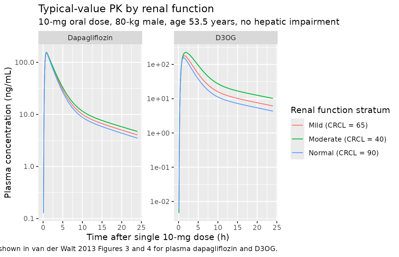
PKNCA validation
For the steady-state simulation we run PKNCA on the 24-hour dosing
interval on day 7 (times 144-168 hours) for each renal-function stratum.
The treatment grouping variable is the cohort label so
per-stratum AUCss can be compared against the paper’s Table 3.
sim_ss_nca <- sim_ss |>
  dplyr::filter(time >= 144, time <= 168) |>
  dplyr::mutate(time_in_interval = time - 144) |>
  dplyr::select(id, time = time_in_interval, Cc, Cc_d3og, cohort)

conc_parent <- PKNCA::PKNCAconc(
  sim_ss_nca |> dplyr::select(id, time, Cc, cohort) |> dplyr::filter(!is.na(Cc)),
  Cc ~ time | cohort + id
)

# One dose row per subject; "time" is reset to 0 (dose at the start of the
# day-7 dosing interval) so PKNCA interprets AUC as AUC over a complete dosing
# interval.
dose_parent <- sim_ss_nca |>
  dplyr::group_by(cohort, id) |>
  dplyr::summarise(time = 0, amt = 10, .groups = "drop")
dose_obj_parent <- PKNCA::PKNCAdose(dose_parent, amt ~ time | cohort + id)

intervals_ss <- data.frame(
  start    = 0,
  end      = 24,
  cmax     = TRUE,
  tmax     = TRUE,
  auclast  = TRUE,
  cmin     = TRUE
)

nca_parent <- PKNCA::pk.nca(
  PKNCA::PKNCAdata(conc_parent, dose_obj_parent, intervals = intervals_ss)
)
knitr::kable(summary(nca_parent),
caption = "Simulated steady-state NCA for dapagliflozin (day-7 interval).")| start | end | cohort | N | auclast | cmax | cmin | tmax |
|---|---|---|---|---|---|---|---|
| 0 | 24 | Mild (CRCL = 65) | 1 | 621 | 157 | 5.59 | 0.750 |
| 0 | 24 | Moderate (CRCL = 40) | 1 | 676 | 159 | 6.63 | 0.750 |
| 0 | 24 | Normal (CRCL = 90) | 1 | 574 | 155 | 4.77 | 0.750 |
conc_metab <- PKNCA::PKNCAconc(
  sim_ss_nca |> dplyr::select(id, time, Cc_d3og, cohort) |> dplyr::filter(!is.na(Cc_d3og)),
  Cc_d3og ~ time | cohort + id
)
dose_obj_metab <- PKNCA::PKNCAdose(dose_parent, amt ~ time | cohort + id)
nca_metab <- PKNCA::pk.nca(
  PKNCA::PKNCAdata(conc_metab, dose_obj_metab, intervals = intervals_ss)
)
knitr::kable(summary(nca_metab),
caption = "Simulated steady-state NCA for D3OG (day-7 interval).")| start | end | cohort | N | auclast | cmax | cmin | tmax |
|---|---|---|---|---|---|---|---|
| 0 | 24 | Mild (CRCL = 65) | 1 | 921 | 188 | 8.51 | 1.50 |
| 0 | 24 | Moderate (CRCL = 40) | 1 | 1410 | 238 | 14.4 | 1.75 |
| 0 | 24 | Normal (CRCL = 90) | 1 | 698 | 162 | 5.91 | 1.25 |
Comparison against published NCA (Table 3)
van der Walt 2013 Table 3 reports steady-state AUC simulations for a 10-mg daily dose stratified by baseline creatinine clearance (Phase I cohort, covariates from MB102007 and MB102027). Numbers in the table are median (95% confidence interval) over 100 simulated trials.
| CrCl stratum | Source AUCss Dapa (ng*h/mL) | Source AUCss D3OG (ng*h/mL) |
|---|---|---|
| 30-49 mL/min | 711 (660, 777) | 1696 (1600, 1864) |
| 50-79 mL/min | 567 (485, 647) | 1133 (1012, 1317) |
| 80-100 mL/min | 526 (260, 822) | 727 (319, 1292) |
Our typical-value simulation is for a single representative subject per stratum (not 100 stochastic trials), so the comparison is order-of-magnitude rather than median-equivalent. The simulated AUC0-24 from the day-7 PKNCA table above should fall within the wide 95% CIs of the source table for the Phase I covariate setting; differences within a factor of 2 are expected given the typical-value simplification and the use of the pooled-cohort reference covariates (WT = 80 kg vs Phase I mean closer to 84 kg, etc.).
Assumptions and deviations
Plasma observations only. The source paper simultaneously fits plasma AND urine concentrations of both dapagliflozin and D3OG. The urine observations and their cumulative-excretion compartments are omitted from this extraction because (i) most downstream nlmixr2lib users want plasma PK only, and (ii) urine modelling adds two extra excretion compartments and two extra residual-error parameters without changing the typical plasma trajectory. Users who need the urine submodel should extend the ODEs in
model()to add d/dt(urine_dapa) and d/dt(urine_d3og) accumulators driven by CLP_renal and CLM respectively.Replicate residual-error cross-correlation dropped. The source paper reports a “replicate” residual error term that captures the within-subject, within-sampling-time correlation between dapagliflozin and D3OG observations – a
theta_replicate * eps_replicateterm shared across the parent and metabolite residual equations (Eqs. 3-4). The standard nlmixr2add() + prop()syntax does not support this kind of cross-output residual cross-correlation. The per-output proportional and additive components are retained at their final-model magnitudes (0.207 / 0.465 for dapa, 0.195 / 0.585 for D3OG); the additional shared term (0.475 in plasma, footnote g) is omitted. The typical-value plasma trajectories and variability quantiles are minimally affected; if you need to add the shared term back, see the Karlsson 1995 paper cited as ref 22 in van der Walt 2013.Bioavailability logit form. The paper uses a logit-transformed BIO parameter so the individual estimate of bioavailability stays in (0, 1). This is reproduced exactly:
logitfdepot <- log(BIO_tv / (1 - BIO_tv))inini()andfdepot <- 1 / (1 + exp(-(logitfdepot + etalogitfdepot)))inmodel(). The IIV onlogitfdepotis reported by the paper as 11.1% CV back-transformed (footnote g); the raw omega on the logit scale is recovered via the delta-method approximationomega ~= (CV / (1 - F_tv))^2giving 0.611.Transit-absorption encoding via
transit()+ fast effective ka. The paper estimates only MTT and N (continuous) for the Savic 2007 closed-form transit-chain absorption (Eq. 5, k_TRANSIT = (N+1)/MTT). It does not estimate a separate first-order absorption rate ka. Our encoding follows the Wilkins 2008 rifampicin pattern:transit(nn, mtt, fdepot)feeds the depot compartment, depot absorbs into central at rate ka, withka = 60 / h(t1/2 in depot ~= 0.012 h = 0.7 min, well below MTT = 0.475 h). The depot exponential is negligible at this rate, so the central-input rate tracks the transit() gamma-PDF directly; the choice is mathematically equivalent to letting transit() feed central without an intermediate depot step but lets us re-use the standard rxode2 transit() / depot /f(depot) = 0pattern that is well-tested across other nlmixr2lib transit absorption models.D3OG carries dapagliflozin mass-equivalents. The metabolite state is driven by the parent’s CLP_M15 flux at the molar 1:1 stoichiometry imposed by glucuronidation; the resulting amount in the D3OG compartment is therefore on the dapagliflozin-mass scale. V2M and CLM as reported in the paper absorb the implicit MW conversion factor (dapagliflozin MW 408.87 g/mol vs D3OG MW 585.0 g/mol), so the same
central_d3og / vc_d3ogratio yields D3OG-mass concentrations in ng/mL that match the paper’s observed plasma D3OG. This is the NONMEM convention used by the source publication.CRCL units. The source
CL_cr,IBWcolumn is in mL/min and is NOT BSA-normalized. The canonicalCRCLregister entry allows non-BSA- normalized usage when documented incovariateData[[CRCL]]$notes(see theCLCRsource alias for the Delattre 2010 amikacin precedent). The CLP_renal coefficientlth_cl_renal = log(0.00310)and the CLM coefficientlth_cl_d3og = log(0.0799)are in (L/h)/(mL/min) – they multiply CRCL directly to give a clearance in L/h.Female-sex shift applied uniformly to each CLP component. The paper states that “In females, CLP and CLM were 16.7 and 19.6% lower” – where CLP refers to total dapagliflozin clearance, the sum of CLP_renal, CLP_M15, and CLP_other. We implement this by multiplying each of the three components by
(1 + e_female_cl * SEXF), which gives the same 16.7% reduction to the total. This matches the NONMEM convention of applying a single typical-value coefficient to the parent-clearance expression as a whole.Hepatic-impairment classification. The source paper uses the Child- Pugh classification (Class A mild, B moderate, C severe) rather than the NCI ODWG classification that the canonical
HEPIMP_SEVandHEPIMP_MODSEVcolumns default to. We reuse theHEPIMP_SEV/HEPIMP_MODSEVcanonical names with the per-modelnotesdocumenting the Child-Pugh basis (seeinst/references/covariate-columns.mdHEPIMP_SEV and HEPIMP_MODSEV entries, source aliases). The two indicators are nested: a Child-Pugh C subject carries both HEPIMP_SEV = 1 and HEPIMP_MODSEV = 1; a Child-Pugh B subject carries HEPIMP_SEV = 0 and HEPIMP_MODSEV = 1. The covariate-effect application accounts for this nesting – effects pile up rather than competing.