Haloperidol (Franken 2017)
Source:vignettes/articles/Franken_2017_haloperidol.Rmd
Franken_2017_haloperidol.RmdModel and source
- Citation: Franken LG, Mathot RAA, Masman AD, Baar FPM, Tibboel D, van Gelder T, Koch BCP, de Winter BCM. Population pharmacokinetics of haloperidol in terminally ill adult patients. Eur J Clin Pharmacol. 2017;73(10):1271-1277. doi:10.1007/s00228-017-2283-6.
- Description: One-compartment population PK model for haloperidol in 28 terminally ill adult palliative-care patients (Franken 2017). Two parallel first-order absorption routes (oral and subcutaneous) with route-specific absorption rate constants fixed from literature (Ka oral = 0.236 1/h, Ka SC = 20 1/h derived from intramuscular Tmax = 20 min). Oral bioavailability F = 0.861 is estimated; SC F is assumed to be 1. IIV is included on F, CL, and Vd; the IIV on F and CL was 99% correlated and is encoded with correlation fixed to unity (BLOCK pattern). Residual variability is additive on log-transformed concentrations (LTBS). Covariate analysis (body weight, age, sex, primary diagnosis, plasma creatinine, urea, bilirubin, GGT, ALP, ALT, AST, CRP, albumin, concomitant CYP2D6 / CYP3A inducers and inhibitors, time-to-death) did not retain any covariate in the final model.
- Article: https://doi.org/10.1007/s00228-017-2283-6
Population
The published analysis included 28 terminally ill adult patients
admitted to the Laurens Cadenza palliative care centre in Rotterdam, the
Netherlands, over a 2-year period. Median age was 69.5 years (range
43-93); 53.6% were male; 92.9% were Caucasian and 7.1% Afro-Caribbean;
all 28 patients had advanced malignancy as the primary diagnosis (89.3%
with epithelial-tissue primary site). Median body weight was 67 kg
(range 35-108); body weight was unknown for about 35% of subjects (the
population median 67 kg was imputed during covariate testing, but
allometric scaling was not retained in the final model). Median duration
of admittance was 18.6 days (range 1.5-176.6). Oral haloperidol doses
ranged 0.5-2 mg/day (tablets or liquid) and subcutaneous bolus doses
0.5-5 mg/day, administered per Dutch national palliative guidelines for
delirium. Eighty-seven sparse plasma samples (median 3 per subject,
range 1-9) were drawn by venous puncture or indwelling catheter and
analysed by LC-MS/MS over a validated range of 0.5-125 ug/L (LLOQ 0.5
ug/L). See Franken 2017 Table 1 for the full baseline summary; the same
information is available programmatically via
readModelDb("Franken_2017_haloperidol")$population.
Source trace
The per-parameter origin is recorded as an in-file comment next to
each ini() entry in
inst/modeldb/specificDrugs/Franken_2017_haloperidol.R. The
table below collects them in one place.
| Equation / parameter | Final value | Source location |
|---|---|---|
lka_oral (Ka oral) |
0.236 1/h (FIXED) | Table 2, footnote a (literature [21]) |
lka_sc (Ka subcutaneous) |
20 1/h (FIXED) | Table 2, footnote a (derived from IM Tmax = 20 min) |
lfdepot (F oral) |
0.861 | Table 2 Final |
lcl (CL) |
29.3 L/h | Table 2 Final |
lvc (Vd) |
1260 L | Table 2 Final |
etalfdepot, etalcl (IIV F and CL, rho =
1) |
55% / 43% CV | Table 2 Final + Section “Structural model” |
etalvc (IIV Vd) |
70% CV | Table 2 Final |
expSd (residual SD on log scale) |
sqrt(0.258) | Table 2 Final (LTBS variance) |
| Equation: 1-compartment model with two parallel first-order absorption depots | n/a | Section “Structural model” + Section “Population pharmacokinetic method” |
| Assumption: SC bioavailability = 1 | n/a | Section “Population pharmacokinetic method” (citation [16]) |
Virtual cohort
Original observed concentrations are not publicly available. The simulation below uses a virtual cohort that mirrors the published Figure 2 scenario: 1000 virtual patients receiving 0.5 mg subcutaneous haloperidol every 12 h over a 72 h window, drawn with between-subject variability from the model’s omega matrix.
set.seed(20170705)

n_subj <- 1000

events <- tibble::tibble(id = seq_len(n_subj)) |>
  tidyr::expand_grid(
    tibble::tribble(
      ~time, ~amt, ~evid, ~cmt,
        0,   0.5, 1L, "depot",
       12,   0.5, 1L, "depot",
       24,   0.5, 1L, "depot",
       36,   0.5, 1L, "depot",
       48,   0.5, 1L, "depot",
       60,   0.5, 1L, "depot"
    )
  )

obs_times <- seq(0, 72, by = 0.5)
obs_events <- tibble::tibble(id = seq_len(n_subj)) |>
  tidyr::expand_grid(
    tibble::tibble(time = obs_times, amt = NA_real_, evid = 0L, cmt = "Cc")
  )

events <- dplyr::bind_rows(events, obs_events) |>
  dplyr::arrange(id, time, dplyr::desc(evid))
Simulation
The model defines depot (SC, cmt = 1),
depot2 (oral, cmt = 2), and central (cmt = 3).
Subcutaneous bioavailability is structurally 1 (the SC depot’s
f defaults to 1); oral bioavailability F = 0.861 is applied
via f(depot2) <- f_oral. The Figure 2 scenario doses
only the SC depot.
mod <- readModelDb("Franken_2017_haloperidol")
sim <- rxode2::rxSolve(mod, events = events) |> as.data.frame()
#> Warning: corrected 'omega' to be a symmetric, positive definite matrix
For deterministic typical-value replications (without between-subject variability or residual error), zero out the random effects:
mod_typical <- mod |> rxode2::zeroRe()
events_typical <- events |> dplyr::filter(id == 1)
sim_typical <- rxode2::rxSolve(mod_typical, events = events_typical) |>
  as.data.frame()
#> ℹ omega/sigma items treated as zero: 'etalfdepot', 'etalcl', 'etalvc'
Replicate published figures
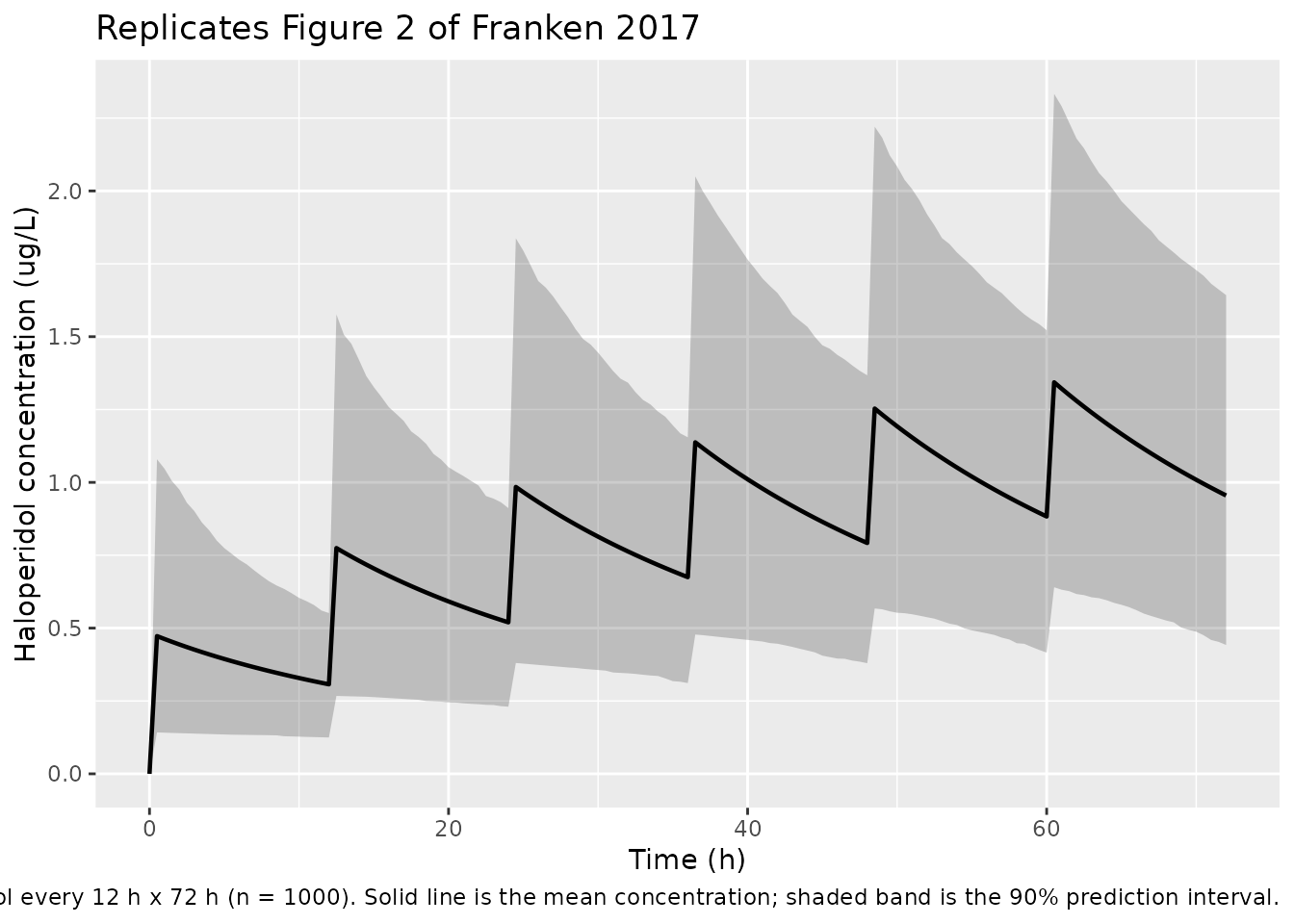
Figure 2: 0.5 mg SC haloperidol every 12 h x 72 h, 1000 simulated patients
Franken 2017 Figure 2 plots the mean haloperidol concentration with the 90% prediction interval over 72 h after 0.5 mg subcutaneously every 12 h.
summary_band <- sim |>
  dplyr::group_by(time) |>
  dplyr::summarise(
    Q05 = stats::quantile(Cc, 0.05, na.rm = TRUE),
    Q50 = mean(Cc, na.rm = TRUE),
    Q95 = stats::quantile(Cc, 0.95, na.rm = TRUE),
    .groups = "drop"
  )

ggplot(summary_band, aes(x = time, y = Q50)) +
  geom_ribbon(aes(ymin = Q05, ymax = Q95), alpha = 0.25) +
  geom_line(linewidth = 0.8) +
  labs(
    x = "Time (h)",
    y = "Haloperidol concentration (ug/L)",
    title = "Replicates Figure 2 of Franken 2017",
    caption = paste(
      "0.5 mg subcutaneous haloperidol every 12 h x 72 h (n = 1000).",
      "Solid line is the mean concentration; shaded band is the 90% prediction interval."
    )
  )
Terminal half-life check
Franken 2017 Discussion: “the t1/2 of around 30 h from our study”. With typical-value CL = 29.3 L/h and Vd = 1260 L, kel = 0.0233 1/h and t1/2 = ln(2) / kel.
cl  <- 29.3
vd  <- 1260
kel <- cl / vd
t_half <- log(2) / kel
data.frame(
  CL_L_per_h = cl,
  Vd_L       = vd,
  kel_per_h  = kel,
  t_half_h   = t_half
) |>
  knitr::kable(
    digits   = c(1, 0, 4, 1),
    caption  = "Terminal half-life from typical-value CL and Vd (paper: ~30 h)."
)| CL_L_per_h | Vd_L | kel_per_h | t_half_h |
|---|---|---|---|
| 29.3 | 1260 | 0.0233 | 29.8 |
PKNCA validation
PKNCA-based NCA over the steady-state 60-72 h interval of the Figure 2 scenario. The “treatment” grouping is added as a single level because Figure 2 covers a single dose regimen; the grouping is retained for compatibility with the standard recipe.
sim_nca <- sim |>
  dplyr::filter(!is.na(Cc), time >= 60, time <= 72) |>
  dplyr::mutate(treatment = "0.5 mg SC q12h") |>
  dplyr::select(id, time, Cc, treatment)

dose_df <- events |>
  dplyr::filter(evid == 1L, time == 60) |>
  dplyr::mutate(treatment = "0.5 mg SC q12h") |>
  dplyr::select(id, time, amt, treatment)

conc_obj <- PKNCA::PKNCAconc(
  sim_nca, Cc ~ time | treatment + id,
  concu = "ug/L", timeu = "h"
)
dose_obj <- PKNCA::PKNCAdose(
  dose_df, amt ~ time | treatment + id, doseu = "mg"
)

intervals_ss <- data.frame(
  start         = 60,
  end           = 72,
  cmax          = TRUE,
  tmax          = TRUE,
  auclast       = TRUE,
  cmin          = TRUE,
  cav           = TRUE
)

nca_res <- PKNCA::pk.nca(
  PKNCA::PKNCAdata(conc_obj, dose_obj, intervals = intervals_ss)
)
knitr::kable(
  as.data.frame(summary(nca_res)),
  caption = "Simulated NCA across the steady-state 60-72 h dosing interval."
)| Interval Start | Interval End | treatment | N | AUClast (h*ug/L) | Cmax (ug/L) | Cmin (ug/L) | Tmax (h) | Cav (ug/L) |
|---|---|---|---|---|---|---|---|---|
| 60 | 72 | 0.5 mg SC q12h | 1000 | 12.5 [39.7] | 1.23 [42.2] | 0.806 [43.4] | 0.500 [0.500, 0.500] | 1.04 [39.7] |
Numeric check: steady-state Cavg from CL and dose rate
For 0.5 mg q12h SC with F = 1, the steady-state average concentration is Cavg_ss = (F * Dose) / (CL * tau). Independent verification against the PKNCA-derived Cavg confirms internal consistency.
dose_mg <- 0.5
tau_h   <- 12
F_sc    <- 1
cl_L_h  <- 29.3

cavg_mg_per_L  <- (F_sc * dose_mg) / (cl_L_h * tau_h)
cavg_ug_per_L  <- cavg_mg_per_L * 1000

data.frame(
  F_sc           = F_sc,
  dose_mg        = dose_mg,
  tau_h          = tau_h,
  CL_L_per_h     = cl_L_h,
  Cavg_ss_ug_L   = cavg_ug_per_L
) |>
  knitr::kable(
    digits  = c(2, 2, 0, 1, 4),
    caption = "Cavg at steady state from Cavg = F * Dose / (CL * tau)."
)| F_sc | dose_mg | tau_h | CL_L_per_h | Cavg_ss_ug_L |
|---|---|---|---|---|
| 1 | 0.5 | 12 | 29.3 | 1.4221 |
Assumptions and deviations
-
Residual-error interpretation. Franken 2017 Methods
reports residual variability as “additive residual error on logarithmic
transformed concentrations” with Table 2 Final value 0.258 and no
explicit units. The packaged model interprets this as a NONMEM
$SIGMAvariance on the log scale (the convention used by the same authors in Franken 2015 morphine) and supplies its square root to rxode2’slnorm()residual model so thatlog(Cobs) - log(Cpred) ~ N(0, expSd^2). If a future reading determines the value was already reported as a log-scale SD,expSdshould be set to 0.258 directly (without the square root). - IIV correlation between F and CL encoded as a BLOCK with rho = 1. The paper section “Structural model” states that the IIV on CL and F showed a 99% correlation and was “fixed to unity with the addition of an extra theta.” The packaged model encodes the equivalent BLOCK(2) structure: variances log(1 + 0.55^2) and log(1 + 0.43^2) with off-diagonal sqrt(var_F * var_CL), which gives an exact correlation of 1. This is mathematically equivalent to the published shared-eta-with-scaling-theta parameterisation.
- Absorption rate constants fixed from literature. Both Ka values were fixed because of insufficient absorption-phase data in the dataset (Table 2 footnote a). Oral Ka = 0.236 1/h is from a prior haloperidol PK study, and SC Ka = 20 1/h was derived by the authors from an intramuscular Tmax of 20 min (no SC literature exists for the intravenously formulated drug used here). The paper notes that halving Ka SC did not affect the other parameters, indicating stability of the remaining estimates with respect to this assumption.
-
Subcutaneous bioavailability assumed to be 1. The
paper assumed F_SC = 1 (“Population pharmacokinetic method”, citation
[16]). The packaged model encodes this by leaving the SC depot’s
bioavailability at the rxode2 default (1), so the estimated
f_oralapplies only to the oral depot viaf(depot2) <- f_oral. - No covariates retained in the final model. The published forward inclusion identified body weight (allometric exponents 0.75 on CL and 1 on Vd) and plasma bilirubin as candidates significant on Vd, but neither survived backward elimination after sharkplot inspection showed that one or two influential subjects accounted for the OFV drop. The packaged model therefore contains no covariate effects, in line with Table 2. Body weight, plasma bilirubin, age, sex, primary diagnosis, plasma creatinine, urea, GGT, ALP, ALT, AST, CRP, albumin, time-to-death, and concomitant CYP2D6 / CYP3A inducers and inhibitors were all tested as covariates but none were retained.
- Body weight missing for ~35% of subjects. Per Franken 2017, weight was not registered for all patients (the hospice protocol did not routinely weigh patients for dosing purposes). When the allometric model was tested, missing weights were imputed at the population median of 67 kg; because allometric scaling was not retained in the final model, this imputation is moot for the packaged model but is recorded here for reproducibility.
- BQL handling. 26.7% of concentrations were below the limit of quantification; half of these were sampled more than 200 h after the last dose. After discarding the post-200-h samples, 14.6% BQL remained. The authors evaluated the Beal M3 method but used M1 (discard) in the final model because of stability problems; the packaged model does not re-implement BQL handling (parameter estimates are reported as-is from the M1 fit).
-
Single dose route per dose record. The model
defines
depot(SC, cmt = 1) anddepot2(oral, cmt = 2). A dosing record selects the route by itscmtvalue; mixed-route patients in the source data were handled by their per-record cmt assignment in NONMEM ADVAN5.