Anti-CD19 CAR T-cell subsets and immunophenotypes, Liso-cel and CAT19 (Salem 2023)
Source:vignettes/articles/Salem_2023_CART_subsets_immunophenotypes.Rmd
Salem_2023_CART_subsets_immunophenotypes.RmdModel and source
- Citation: Salem AM, Mugundu GM, Singh AP (2023). Development of a multiscale mechanistic modeling framework integrating differential cellular kinetics of CAR T-cell subsets and immunophenotypes in cancer patients. CPT Pharmacometrics Syst Pharmacol 12(9):1285-1296.
- Article: https://doi.org/10.1002/psp4.13009 (open access, PMC10508581)
- Equations: Appendix S1; Monolix model code: Appendix S2.
Salem et al. extend the multiscale cellular-kinetic / pharmacodynamic
(CK-PD) model of Singh et al. 2021
(Singh_2021_idecabtageneVicleucel_human) to anti-CD19 CAR T
cells, in three sequential steps. Each step is a separately fitted
model, so the paper contributes five model files:
| Step | Model | Data |
|---|---|---|
| 1 |
Salem_2023_CART_FMC63_invitro_qsp,
Salem_2023_CART_CAT19_invitro_qsp
|
4-h cytotoxicity of FMC63- and CAT19-binder CAR T cells against SupT1 CD19+ cells |
| 2 | Salem_2023_lisocabtageneMaraleucel_qsp |
Mean / median Liso-cel flow cytometry and qPCR in adult DLBCL and ALL |
| 2 | Salem_2023_CART_CAT19_qsp |
Individual CAT19 flow cytometry and qPCR in 14 children with ALL |
| 3 | Salem_2023_CART_CAT19_immunophenotype_qsp |
Step 2 CAT19 data plus immunophenotype percentages in 4 of the 14 children |
In every clinical model the infused CAR T cells distribute between blood and bone marrow; CARs bind CD19 on tumour cells to form CAR-target complexes; the number of complexes per CAR T cell drives Emax expansion and the number of complexes per tumour cell drives Emax killing. Step 2 splits the product into CD4+ and CD8+ subsets with their own expansion rates, and step 3 further splits each subset into stem-cell memory (TSCM), central memory (TCM), effector memory (TEM) and terminal effector (TEFF) cells.
nms <- c(
  "Salem_2023_CART_FMC63_invitro_qsp",
  "Salem_2023_CART_CAT19_invitro_qsp",
  "Salem_2023_lisocabtageneMaraleucel_qsp",
  "Salem_2023_CART_CAT19_qsp",
  "Salem_2023_CART_CAT19_immunophenotype_qsp"
)
uis <- lapply(nms, function(n) rxode2::rxode(readModelDb(n)))
#> ℹ parameter labels from comments will be replaced by 'label()'
#> ℹ parameter labels from comments will be replaced by 'label()'
#> ℹ parameter labels from comments will be replaced by 'label()'
names(uis) <- nms
Population
- In vitro (step 1). SupT1 cells engineered to express CD19, cocultured with FMC63- or CAT19-binder CAR T cells at effector:target ratios of 0.4:1 to 6.4:1 (5000 tumour cells in 175 uL); percent lysis at 4 h digitised from Ghorashian et al. 2019 (Nat Med 25:1408-1414).
- Liso-cel (step 2). Summary-level data (Table 1 of the paper): mean +/- SEM blood CAR+CD4+ and CAR+CD8+ cells/uL in adult ALL after 2 x 10^5 or 2 x 10^6 cells/kg (Turtle et al. 2016; n = 13 and 15; a 70 kg weight was assumed to convert the doses), and median blood CAR+CD3+/CD4+/CD8+ cells/uL (50 x 10^6 cells, n = 45) and median qPCR transgene copies/ug genomic DNA (50, 100 and 150 x 10^6 cells, n = 45, 176 and 41) in adult DLBCL from the Breyanzi FDA review. The product is 1:1 CD4:CD8.
- CAT19 (steps 2 and 3). 14 children with relapsed / refractory B-ALL in the CARPALL study (Ghorashian et al. 2019) who received a median 1 x 10^6 CAR+ cells/kg; a 30 kg weight was assumed for everyone. Individual flow cytometry (n = 13) and qPCR (n = 14) in blood and bone marrow; the product contained a median 54.65% CD4+ and 37.65% CD8+ CAR T cells. Immunophenotype percentages before infusion and up to 1080 days after it were available for 4 patients (Biasco et al. 2021, Nat Cancer 2:629-642): two with a highly polyclonal product and long persistence (patients 4 and 6) and two with low polyclonality and short persistence (patients 10 and 17).
lapply(uis, function(u) u$population[c("species", "n_subjects", "disease_state")])
#> $Salem_2023_CART_FMC63_invitro_qsp
#> $Salem_2023_CART_FMC63_invitro_qsp$species
#> [1] "in vitro (SupT1 CD19+ cell line)"
#>
#> $Salem_2023_CART_FMC63_invitro_qsp$n_subjects
#> [1] NA
#>
#> $Salem_2023_CART_FMC63_invitro_qsp$disease_state
#> [1] "SupT1 cells engineered to express CD19, cocultured with FMC63-binder anti-CD19 CAR T cells"
#>
#>
#> $Salem_2023_CART_CAT19_invitro_qsp
#> $Salem_2023_CART_CAT19_invitro_qsp$species
#> [1] "in vitro (SupT1 CD19+ cell line)"
#>
#> $Salem_2023_CART_CAT19_invitro_qsp$n_subjects
#> [1] NA
#>
#> $Salem_2023_CART_CAT19_invitro_qsp$disease_state
#> [1] "SupT1 cells engineered to express CD19, cocultured with low-affinity CAT19-binder anti-CD19 CAR T cells"
#>
#>
#> $Salem_2023_lisocabtageneMaraleucel_qsp
#> $Salem_2023_lisocabtageneMaraleucel_qsp$species
#> [1] "human"
#>
#> $Salem_2023_lisocabtageneMaraleucel_qsp$n_subjects
#> [1] NA
#>
#> $Salem_2023_lisocabtageneMaraleucel_qsp$disease_state
#> [1] "Relapsed / refractory diffuse large B-cell lymphoma (Breyanzi BLA, TRANSCEND NHL 001) and adult B-cell acute lymphoblastic leukaemia (Turtle et al. 2016)"
#>
#>
#> $Salem_2023_CART_CAT19_qsp
#> $Salem_2023_CART_CAT19_qsp$species
#> [1] "human"
#>
#> $Salem_2023_CART_CAT19_qsp$n_subjects
#> [1] 14
#>
#> $Salem_2023_CART_CAT19_qsp$disease_state
#> [1] "Relapsed / refractory paediatric B-cell acute lymphoblastic leukaemia (CARPALL study, Ghorashian et al. 2019)"
#>
#>
#> $Salem_2023_CART_CAT19_immunophenotype_qsp
#> $Salem_2023_CART_CAT19_immunophenotype_qsp$species
#> [1] "human"
#>
#> $Salem_2023_CART_CAT19_immunophenotype_qsp$n_subjects
#> [1] 14
#>
#> $Salem_2023_CART_CAT19_immunophenotype_qsp$disease_state
#> [1] "Relapsed / refractory paediatric B-cell acute lymphoblastic leukaemia (CARPALL study)"
Source trace
Every ini() value carries an in-file comment naming its
source. Summary:
| Element | Value(s) | Source |
|---|---|---|
| In vitro binding / kill ODEs | – | Appendix S1 Eqs. 1-5; Appendix S2 Figure 1 code |
| KKillMax, KC50CAR-T in vitro (FMC63 / CAT19) | 0.24, 0.22 /h; 9.16, 0.28 complexes/cell | Table 2, in vitro |
| DTTumor, DTCAR-T, AgTumor, AgCAR, Tumor0, Vwell | 30 h, 24 h, 4000, 15000, 5000 cells, 175 uL | Table 2, in vitro |
| Kon / Koff (FMC63 / CAT19) | 2.07E5, 2.15E5 /M/s; 6.81E-5, 0.003 /s | Table 2 |
| Clinical CK ODEs (effector / memory, CD4 / CD8, blood / marrow) | – | Appendix S1 Eqs. 6-17; Appendix S2 Figure 2 code |
| Binding, expansion, kill and tumour ODEs | – | Appendix S1 Eqs. 19-42 |
| Liso-cel KmaxExpCD8 / CD4, Rm, Kelm, K12, K21, KKillMax | 2.14, 1.92, 7E-6, 0.024, 0.4, 0.15, 1.8 /day | Table 2, Liso-cel |
| EC50Exp, Kele | 10 complexes/cell, 113 /day | Table 2 (fixed from Singh 2021) |
| Disease-specific AgTumor, DTTumor, ICTumorBM, ICTumorPB (DLBCL / ALL) | 20000 / 4000; 29 / 5.8 day; 5E10 / 1.06E11; 0 / 5.5E9 cells/L | Table 2, Liso-cel |
| Kmigration, Vb, Vbm | 0.001 /day, 5 L, 1.6 L | Table 2 |
| qPCR link (Liso-cel) | ln(copies) = 7.62 + 0.85 ln(cells/uL) | Eq. 1, Table 2; Appendix S2 code 7.6204 / 0.8537 |
| CAT19 KmaxExpCD8, Rm, Kelm, K12 | 5.3, 0.000037, 0.013, 0.11 /day | Results text (Table 2 per month: 159, 0.001, 0.39, 3.3) |
| CAT19 K21, KmaxExpCD4 ratio, PCTCD8 / PCTCD4 | 0.176 /day, 1.12, 38 / 54% | Table 2, CAT19 |
| CAT19 qPCR link | intercept 7.26, slope 0.74 | Table 2, CAT19 |
| CAT19 omegas (KmaxExpCD8, PCT, Rm, Kelm, K12, K21) | 0.4, 0.5, 5.04, 1.35, 2.08, 1.08 | Table 2, CAT19 |
| Immunophenotype ODEs | – | Appendix S1 Eqs. 43-66 |
| Step 3 KmaxExpCD8, Rm1, Rm2, Rm3 | 3.44, 0.26, 0.4, 0.29 /day | Table 2, step 3 |
| Polyclonality effects on Rm1-Rm3 | x 0.08, 0.21, 0.19 | Table 2, step 3; Discussion (92%, 79%, 81% reductions) |
| Step 3 omegas (KmaxExpCD8, Rm1-3, Kelm, K12, K21) | 0.4, 0.2, 1.35, 2.08, 1.08 (all fixed) | Table 2, step 3 |
Step 1: in vitro killing (Figure 1b)
Each well is seeded with 5000 SupT1 CD19+ cells and
E:T x 5000 CAR T cells; lysis is read at 4 h.
et_ratio <- c(6.4, 3.2, 1.6, 0.8, 0.4)

invitro_lysis <- function(ui, ratio) {
  ids <- seq_along(ratio)
  d <- rbind(
    data.frame(id = ids, time = 0, amt = 5000, evid = 1, cmt = "tumor"),
    data.frame(id = ids, time = 0, amt = 5000 * ratio, evid = 1, cmt = "cart"),
    data.frame(id = ids, time = 4, amt = 0, evid = 0, cmt = "tumor")
  )
  d <- d[order(d$id, d$time, -d$evid), ]
  s <- as.data.frame(rxode2::rxSolve(ui, d))
  if (is.null(s$id)) s$id <- 1L
  s$lysis[match(seq_along(ratio), s$id)]
}

invitro <- data.frame(
  construct = rep(c("CAT19", "FMC63"), each = length(et_ratio)),
  et_ratio = rep(et_ratio, 2),
  simulated = c(
    invitro_lysis(uis$Salem_2023_CART_CAT19_invitro_qsp, et_ratio),
    invitro_lysis(uis$Salem_2023_CART_FMC63_invitro_qsp, et_ratio)
  ),
  # Model-fitted lines of Figure 1b, read by the maintainers at each E:T ratio.
  published_fit = c(47.5, 41.5, 32.5, 22, 11, 42.5, 33, 21.5, 11, 3)
)
invitro$diff <- invitro$simulated - invitro$published_fit

invitro |>
  dplyr::mutate(simulated = round(simulated, 1), diff = round(diff, 1)) |>
  dplyr::rename(
    "Construct" = construct, "E:T ratio" = et_ratio,
    "Simulated lysis (%)" = simulated, "Figure 1b fit (%)" = published_fit,
    "Difference (points)" = diff
  ) |>
knitr::kable()| Construct | E:T ratio | Simulated lysis (%) | Figure 1b fit (%) | Difference (points) |
|---|---|---|---|---|
| CAT19 | 6.4 | 47.0 | 47.5 | -0.5 |
| CAT19 | 3.2 | 41.0 | 41.5 | -0.5 |
| CAT19 | 1.6 | 32.1 | 32.5 | -0.4 |
| CAT19 | 0.8 | 21.2 | 22.0 | -0.8 |
| CAT19 | 0.4 | 10.5 | 11.0 | -0.5 |
| FMC63 | 6.4 | 41.7 | 42.5 | -0.8 |
| FMC63 | 3.2 | 32.8 | 33.0 | -0.2 |
| FMC63 | 1.6 | 21.8 | 21.5 | 0.3 |
| FMC63 | 0.8 | 10.9 | 11.0 | -0.1 |
| FMC63 | 0.4 | 2.5 | 3.0 | -0.5 |
# Deterministic solve against values read off a figure: a wrong KKillMax,
# KC50 or binding constant moves the curve by many lysis points.
stopifnot(all(abs(invitro$diff) < 3))
# Replicates Figure 1b of Salem 2023.
invitro$et_lbl <- factor(paste0(invitro$et_ratio, ":1"), levels = paste0(rev(et_ratio), ":1"))
ggplot(invitro, aes(et_lbl)) +
  geom_line(aes(y = simulated, group = construct)) +
  geom_point(aes(y = published_fit), shape = 1, colour = "red", size = 2) +
  facet_wrap(~construct) +
  labs(
    x = "E:T ratio", y = "% lysis at 4 h",
    title = "Figure 1b - model (line) vs published fit (circles)"
  )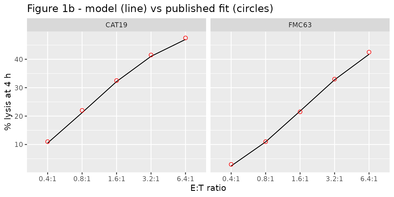
The ~33-fold lower KC50 of the low-affinity CAT19 binder offsets its ~40-fold faster dissociation, so the two constructs kill SupT1 cells with similar potency in this assay.
Step 2: Liso-cel in adult DLBCL and ALL (Figure 2b)
A dose is the total number of CAR+ T cells, given as one record on
each subset compartment; f() applies the 1:1 split.
liso <- rxode2::zeroRe(uis$Salem_2023_lisocabtageneMaraleucel_qsp)
#> Warning: No sigma parameters in the model

liso_events <- function(total_cells, times, dis_all) {
  ev <- rxode2::et(amt = total_cells, cmt = "carte_cd8_pb")
  ev <- rxode2::et(ev, amt = total_cells, cmt = "carte_cd4_pb")
  ev <- rxode2::et(ev, times, cmt = "carte_cd8_pb")
  d <- as.data.frame(ev)
  d$DIS_ALL <- dis_all
  d
}

tt_short <- sort(unique(c(seq(0, 2, by = 0.02), seq(2, 28, by = 0.25))))
tt_long <- sort(unique(c(tt_short, seq(28, 730, by = 2))))

liso_scen <- data.frame(
  scenario = c("DLBCL 50e6 (BLA)", "ALL 2e5/kg (Turtle DL1)", "ALL 2e6/kg (Turtle DL2)"),
  cells = c(50e6, 2e5 * 70, 2e6 * 70),
  dis_all = c(0, 1, 1)
)
sim_liso <- dplyr::bind_rows(lapply(seq_len(nrow(liso_scen)), function(i) {
  tt <- if (liso_scen$dis_all[i] == 0) tt_long[tt_long <= 180] else tt_short
  s <- as.data.frame(rxode2::rxSolve(liso,
    liso_events(liso_scen$cells[i], tt, liso_scen$dis_all[i]),
    atol = 1e-10, rtol = 1e-8
  ))
  s$scenario <- liso_scen$scenario[i]
  s
}))
#> ℹ omega/sigma items treated as zero: 'etalkkill_max'
#> ℹ omega/sigma items treated as zero: 'etalkkill_max'
#> ℹ omega/sigma items treated as zero: 'etalkkill_max'
sim_liso$scenario <- factor(sim_liso$scenario, levels = liso_scen$scenario)
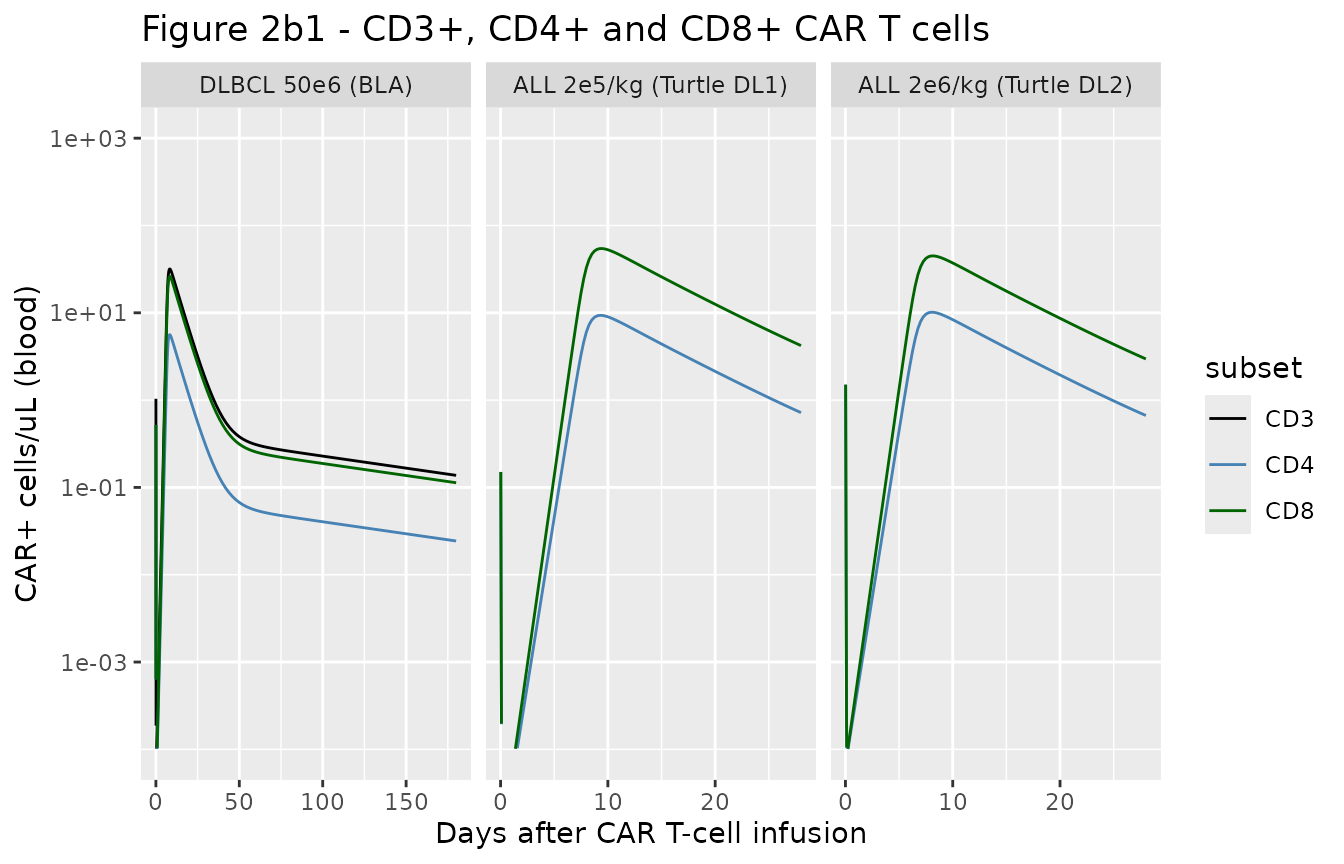
# Replicates Figure 2b1 of Salem 2023 (typical-value lines).
sim_liso |>
  dplyr::filter(time > 0) |>
  dplyr::select(time, scenario, CD3 = cart_cd3_pb, CD4 = cart_cd4_pb, CD8 = cart_cd8_pb) |>
  tidyr::pivot_longer(c(CD3, CD4, CD8), names_to = "subset", values_to = "cells") |>
  dplyr::filter(!(subset == "CD3" & scenario != "DLBCL 50e6 (BLA)")) |>
  ggplot(aes(time, cells, colour = subset)) +
  geom_line() +
  scale_y_log10(limits = c(1e-4, 1e3)) +
  scale_colour_manual(values = c(CD3 = "black", CD4 = "steelblue", CD8 = "darkgreen")) +
  facet_wrap(~scenario, scales = "free_x") +
  labs(
    x = "Days after CAR T-cell infusion", y = "CAR+ cells/uL (blood)",
    title = "Figure 2b1 - CD3+, CD4+ and CD8+ CAR T cells"
  )
bla <- sim_liso[sim_liso$scenario == "DLBCL 50e6 (BLA)", ]
bla_peak <- max(bla$cart_cd3_pb[bla$time > 1])
bla_180 <- bla$cart_cd3_pb[which.min(abs(bla$time - 180))]
c(peak_cd3 = bla_peak, day180_cd3 = bla_180)
#>   peak_cd3 day180_cd3
#> 31.7918128  0.1374849
# Figure 2b1 (BLA, median data and fit): CD3+ peak about 20 cells/uL near
# day 7-10 and about 0.15 cells/uL at day 180. A factor-of-two window still
# fails on a mis-transcribed expansion, conversion or elimination constant.
stopifnot(bla_peak > 10, bla_peak < 40, bla_180 > 0.075, bla_180 < 0.3)
The typical-value DLBCL (BLA) curve follows the published fit to within a factor of about 1.5 (peak CD3+ 32 vs about 20 cells/uL; 0.14 vs about 0.15 cells/uL at day 180). The typical-value ALL curves sit below the Turtle data (peak CD8+ about 50 vs 100 cells/uL at 2 x 10^5 cells/kg, and about 40 vs 400 cells/uL at 2 x 10^6 cells/kg) because in the paper each summary profile carries its own empirical-Bayes value of the 50% random effect on KKillMax; a lower individual kill rate keeps more tumour alive and so drives more expansion.
# Replicates Figure 2b2 of Salem 2023: blood qPCR in DLBCL at three dose levels.
sim_qpcr <- dplyr::bind_rows(lapply(c(50e6, 100e6, 150e6), function(d) {
  s <- as.data.frame(rxode2::rxSolve(liso, liso_events(d, tt_long, 0),
    atol = 1e-10, rtol = 1e-8
  ))
  s$dose <- paste0(d / 1e6, " x10^6 cells")
  s
}))
#> ℹ omega/sigma items treated as zero: 'etalkkill_max'
#> ℹ omega/sigma items treated as zero: 'etalkkill_max'
#> ℹ omega/sigma items treated as zero: 'etalkkill_max'
sim_qpcr |>
  dplyr::filter(time > 0) |>
  ggplot(aes(time, transgene)) +
  geom_line() +
  scale_y_log10(limits = c(1, 1e5)) +
  facet_wrap(~dose, scales = "free_x") +
  labs(
    x = "Days after CAR T-cell infusion", y = "Transgene copies/ug gDNA",
    title = "Figure 2b2 - qPCR in DLBCL (typical value)"
  )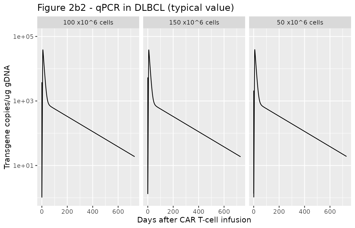
Peak qPCR is nearly flat across the three doses, as in the paper, because expansion is limited by the antigen supply in bone marrow rather than by the dose. The typical-value curves run about two- to three-fold above the individual Figure 2b2 fits, which again carry their own KKillMax values; the paper’s own typical-value simulations (next section) agree with the packaged model to within a few percent.
Typical-value exposure across CD4:CD8 ratios and tumour burden (Appendix S1 Table S1)
Appendix S1 Table S1 reports the typical-value (“mean simulation”) Cmax and AUC(0-28 day) of blood transgene after 50 x 10^6 Liso-cel cells in a DLBCL patient, for CD4:CD8 product ratios from 99:1 to 1:99 at initial bone-marrow tumour burdens of 5E9, 5E10 and 5E11 cells/L. The same grid is simulated here and summarised with PKNCA.
Cmax is taken from day 1 onwards. At time zero the whole dose is in the blood as effector cells, which the 113 /day effector elimination clears within hours; that instant reads about 14,000 copies/ug gDNA for every scenario, whereas Table S1 reports expansion peaks as low as 3603, so the published Cmax is the expansion peak.
ratios <- data.frame(
  ratio = c("99:1", "9:1", "3:1", "1:1", "1:3", "1:9", "1:99"),
  pct_cd4 = c(99, 90, 75, 50, 25, 10, 1)
)
burdens <- c(5e9, 5e10, 5e11)
grid <- tidyr::expand_grid(ratios, tumor_bm0 = burdens)
grid$treatment <- paste0(grid$ratio, ", ", format(grid$tumor_bm0, scientific = TRUE), " cells/L")
tt_nca <- seq(0, 28, by = 0.05)

sim_s1 <- dplyr::bind_rows(lapply(seq_len(nrow(grid)), function(i) {
  s <- as.data.frame(rxode2::rxSolve(liso, liso_events(50e6, tt_nca, 0),
    params = c(
      pct_cd4 = grid$pct_cd4[i], pct_cd8 = 100 - grid$pct_cd4[i],
      tumor_bm0 = grid$tumor_bm0[i]
    ),
    atol = 1e-10, rtol = 1e-8
  ))
  s$id <- i
  s$treatment <- grid$treatment[i]
  s
}))
#> ℹ omega/sigma items treated as zero: 'etalkkill_max'
#> ℹ omega/sigma items treated as zero: 'etalkkill_max'
#> ℹ omega/sigma items treated as zero: 'etalkkill_max'
#> ℹ omega/sigma items treated as zero: 'etalkkill_max'
#> ℹ omega/sigma items treated as zero: 'etalkkill_max'
#> ℹ omega/sigma items treated as zero: 'etalkkill_max'
#> ℹ omega/sigma items treated as zero: 'etalkkill_max'
#> ℹ omega/sigma items treated as zero: 'etalkkill_max'
#> ℹ omega/sigma items treated as zero: 'etalkkill_max'
#> ℹ omega/sigma items treated as zero: 'etalkkill_max'
#> ℹ omega/sigma items treated as zero: 'etalkkill_max'
#> ℹ omega/sigma items treated as zero: 'etalkkill_max'
#> ℹ omega/sigma items treated as zero: 'etalkkill_max'
#> ℹ omega/sigma items treated as zero: 'etalkkill_max'
#> ℹ omega/sigma items treated as zero: 'etalkkill_max'
#> ℹ omega/sigma items treated as zero: 'etalkkill_max'
#> ℹ omega/sigma items treated as zero: 'etalkkill_max'
#> ℹ omega/sigma items treated as zero: 'etalkkill_max'
#> ℹ omega/sigma items treated as zero: 'etalkkill_max'
#> ℹ omega/sigma items treated as zero: 'etalkkill_max'
#> ℹ omega/sigma items treated as zero: 'etalkkill_max'
conc_s1 <- sim_s1 |>
  dplyr::filter(!is.na(transgene)) |>
  dplyr::select(id, time, transgene, treatment)

intervals_s1 <- data.frame(
  start = c(0, 1), end = c(28, 28),
  auclast = c(TRUE, FALSE), cmax = c(FALSE, TRUE)
)
nca_s1 <- PKNCA::pk.nca(PKNCA::PKNCAdata(
  PKNCA::PKNCAconc(conc_s1, transgene ~ time | treatment + id),
  intervals = intervals_s1
))
#> No dose information provided, calculations requiring dose will return NA.

# Appendix S1 Table S1 absolute values.
ref_s1 <- data.frame(
  treatment = grid$treatment,
  cmax = c(
    3603, 25835, 187104, 4010, 28706, 210352, 4585, 32534, 234785,
    5266, 36524, 256942, 5790, 39244, 273884, 6086, 40683, 282166,
    6232, 41363, 285982
  ),
  auclast = c(
    43903, 262801, 1804107, 48085, 292511, 2036330, 54257, 330472, 2296509,
    60584, 366141, 2515404, 65582, 390892, 2653686, 68267, 404269, 2725646,
    69639, 410692, 2758981
  )
)

tab_s1 <- ncaComparisonTable(
  nca_s1, ref_s1,
  by = "treatment",
  units = c(cmax = "copies/ug gDNA", auclast = "copies*day/ug gDNA"),
  tolerance_pct = 20
)
knitr::kable(tab_s1)| NCA parameter | treatment | Reference | Simulated | % diff |
|---|---|---|---|---|
| Cmax (copies/ug gDNA) | 99:1, 5e+09 cells/L | 3600 | 3850 | +7.0% |
| Cmax (copies/ug gDNA) | 99:1, 5e+10 cells/L | 25800 | 27600 | +6.7% |
| Cmax (copies/ug gDNA) | 99:1, 5e+11 cells/L | 187000 | 197000 | +5.5% |
| Cmax (copies/ug gDNA) | 9:1, 5e+09 cells/L | 4010 | 4320 | +7.7% |
| Cmax (copies/ug gDNA) | 9:1, 5e+10 cells/L | 28700 | 30900 | +7.8% |
| Cmax (copies/ug gDNA) | 9:1, 5e+11 cells/L | 210000 | 224000 | +6.7% |
| Cmax (copies/ug gDNA) | 3:1, 5e+09 cells/L | 4580 | 4940 | +7.7% |
| Cmax (copies/ug gDNA) | 3:1, 5e+10 cells/L | 32500 | 34900 | +7.2% |
| Cmax (copies/ug gDNA) | 3:1, 5e+11 cells/L | 235000 | 252000 | +7.3% |
| Cmax (copies/ug gDNA) | 1:1, 5e+09 cells/L | 5270 | 5690 | +8.1% |
| Cmax (copies/ug gDNA) | 1:1, 5e+10 cells/L | 36500 | 39100 | +7.1% |
| Cmax (copies/ug gDNA) | 1:1, 5e+11 cells/L | 257000 | 278000 | +8.2% |
| Cmax (copies/ug gDNA) | 1:3, 5e+09 cells/L | 5790 | 6250 | +8.0% |
| Cmax (copies/ug gDNA) | 1:3, 5e+10 cells/L | 39200 | 41900 | +6.8% |
| Cmax (copies/ug gDNA) | 1:3, 5e+11 cells/L | 274000 | 294000 | +7.3% |
| Cmax (copies/ug gDNA) | 1:9, 5e+09 cells/L | 6090 | 6530 | +7.2% |
| Cmax (copies/ug gDNA) | 1:9, 5e+10 cells/L | 40700 | 43200 | +6.3% |
| Cmax (copies/ug gDNA) | 1:9, 5e+11 cells/L | 282000 | 301000 | +6.6% |
| Cmax (copies/ug gDNA) | 1:99, 5e+09 cells/L | 6230 | 6670 | +7.1% |
| Cmax (copies/ug gDNA) | 1:99, 5e+10 cells/L | 41400 | 43900 | +6.2% |
| Cmax (copies/ug gDNA) | 1:99, 5e+11 cells/L | 286000 | 304000 | +6.4% |
| AUClast (copies*day/ug gDNA) | 99:1, 5e+09 cells/L | 43900 | 37900 | -13.7% |
| AUClast (copies*day/ug gDNA) | 99:1, 5e+10 cells/L | 263000 | 264000 | +0.3% |
| AUClast (copies*day/ug gDNA) | 99:1, 5e+11 cells/L | 1800000 | 1850000 | +2.7% |
| AUClast (copies*day/ug gDNA) | 9:1, 5e+09 cells/L | 48100 | 42400 | -11.8% |
| AUClast (copies*day/ug gDNA) | 9:1, 5e+10 cells/L | 293000 | 295000 | +1.0% |
| AUClast (copies*day/ug gDNA) | 9:1, 5e+11 cells/L | 2040000 | 2100000 | +3.3% |
| AUClast (copies*day/ug gDNA) | 3:1, 5e+09 cells/L | 54300 | 48400 | -10.9% |
| AUClast (copies*day/ug gDNA) | 3:1, 5e+10 cells/L | 330000 | 333000 | +0.6% |
| AUClast (copies*day/ug gDNA) | 3:1, 5e+11 cells/L | 2300000 | 2360000 | +2.8% |
| AUClast (copies*day/ug gDNA) | 1:1, 5e+09 cells/L | 60600 | 55700 | -8.1% |
| AUClast (copies*day/ug gDNA) | 1:1, 5e+10 cells/L | 366000 | 373000 | +1.9% |
| AUClast (copies*day/ug gDNA) | 1:1, 5e+11 cells/L | 2520000 | 2610000 | +3.6% |
| AUClast (copies*day/ug gDNA) | 1:3, 5e+09 cells/L | 65600 | 61000 | -6.9% |
| AUClast (copies*day/ug gDNA) | 1:3, 5e+10 cells/L | 391000 | 400000 | +2.3% |
| AUClast (copies*day/ug gDNA) | 1:3, 5e+11 cells/L | 2650000 | 2760000 | +3.9% |
| AUClast (copies*day/ug gDNA) | 1:9, 5e+09 cells/L | 68300 | 63700 | -6.7% |
| AUClast (copies*day/ug gDNA) | 1:9, 5e+10 cells/L | 404000 | 413000 | +2.1% |
| AUClast (copies*day/ug gDNA) | 1:9, 5e+11 cells/L | 2730000 | 2820000 | +3.6% |
| AUClast (copies*day/ug gDNA) | 1:99, 5e+09 cells/L | 69600 | 65100 | -6.5% |
| AUClast (copies*day/ug gDNA) | 1:99, 5e+10 cells/L | 411000 | 419000 | +2.1% |
| AUClast (copies*day/ug gDNA) | 1:99, 5e+11 cells/L | 2760000 | 2860000 | +3.6% |
pct_s1 <- as.numeric(gsub("[*%+]", "", tab_s1[["% diff"]]))
stopifnot(!anyNA(pct_s1), length(pct_s1) == 42)
c(median_abs = median(abs(pct_s1)), max_abs = max(abs(pct_s1)))
#> median_abs    max_abs
#>        6.7       13.7
# Deterministic typical-value solves against the paper's own typical-value
# table. Realised: median |diff| 6.7%, maximum 13.7% (AUC at the lowest tumour
# burden). A mis-transcribed expansion, conversion, binding or qPCR constant
# shifts these exposures by tens of percent.
stopifnot(median(abs(pct_s1)) < 10, max(abs(pct_s1)) < 20)
All 42 exposures agree within 14%. Cmax runs a uniform 6-8% above Table S1, and AUC agrees within 4% except at the lowest tumour burden (7-14% below). Both patterns fit a coarser time grid in the published simulation: a grid that steps over the expansion peak under-reads Cmax, and one that steps over the steep post-infusion fall over-reads the early AUC. That early contribution matters most when expansion is smallest. The ratios to the 1:1 reference (Table S1 “Ratio” columns) are reproduced as well: a CD8+-rich product gives higher Cmax and AUC, with diminishing returns beyond 1:1, and a higher tumour burden drives more expansion.
Step 2: CAT19 in children with ALL (Figure 4)
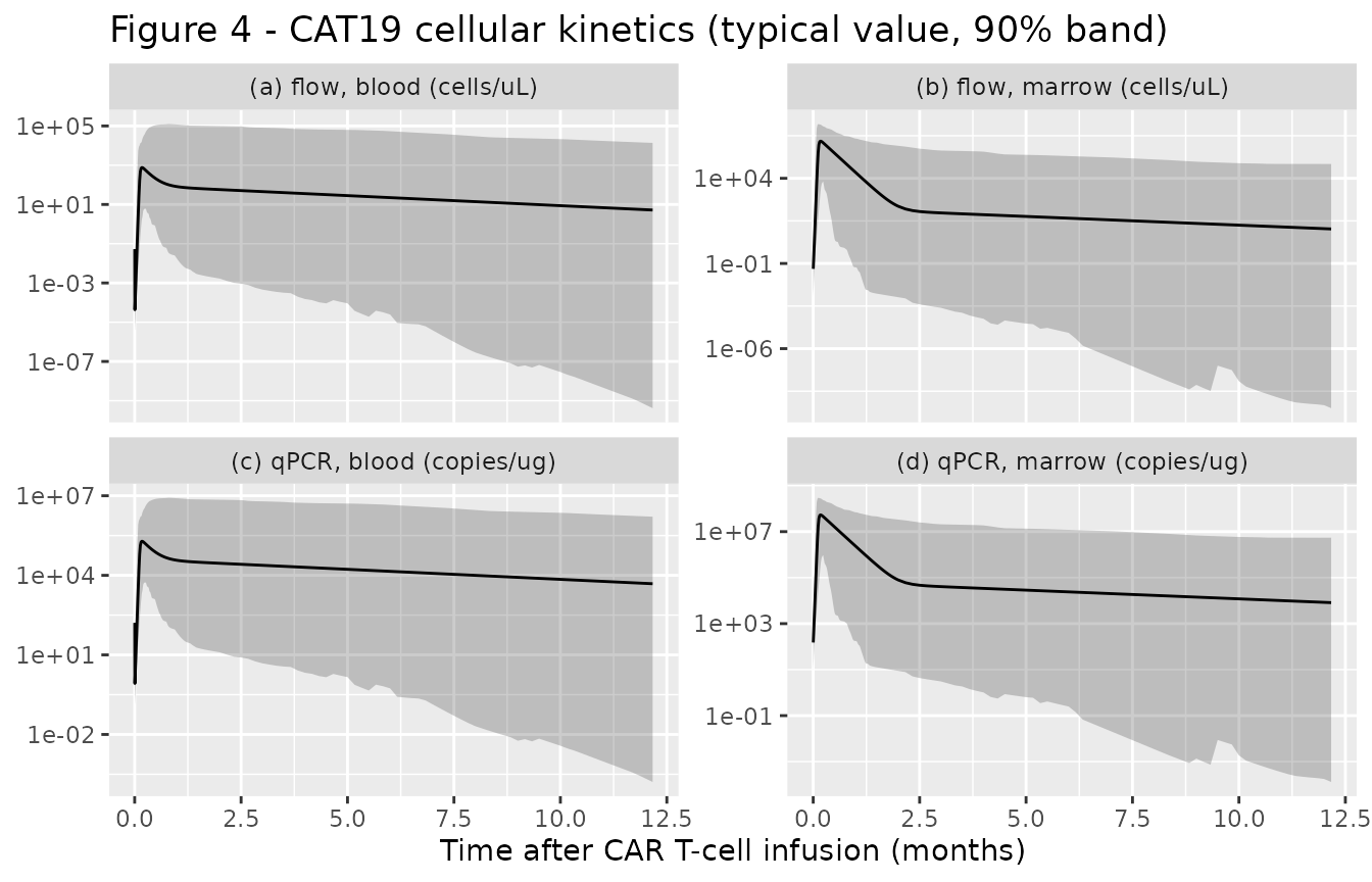
The CAT19 model carries between-subject variability on CD8+ expansion, the CD4 / CD8 product fractions, conversion to memory, memory elimination and distribution. A virtual cohort of 200 children at the source’s assumed 30 kg receives 1 x 10^6 CAR+ cells/kg.
cat19 <- uis$Salem_2023_CART_CAT19_qsp
wt <- 30
dose_cat19 <- 1e6 * wt
tt_cat19 <- sort(unique(c(seq(0, 2, by = 0.05), seq(2, 60, by = 0.5), seq(60, 365, by = 5))))

cat19_events <- function(n, times) {
  ev <- rxode2::et(amt = dose_cat19, cmt = "carte_cd8_pb")
  ev <- rxode2::et(ev, amt = dose_cat19, cmt = "carte_cd4_pb")
  ev <- rxode2::et(ev, times, cmt = "carte_cd8_pb")
  ev <- rxode2::et(ev, id = seq_len(n))
  d <- as.data.frame(ev)
  d$WT <- wt
  d
}

sim_cat19_tv <- as.data.frame(rxode2::rxSolve(rxode2::zeroRe(cat19), cat19_events(1, tt_cat19),
  atol = 1e-10, rtol = 1e-8
))
#> Warning: No sigma parameters in the model
#> ℹ omega/sigma items treated as zero: 'etalkexp_max_cd8', 'etalpct_cd8', 'etalpct_cd4', 'etalrm', 'etalkel_m', 'etalk12', 'etalk21'

rxode2::rxSetSeed(20231009)
# A few sampled non-responders (a very low Rm or K12 with a high K21) leave the
# tumour uncontrolled; it then regrows exponentially without bound (the model
# has no carrying capacity), past 1e19 cells/L in blood within the year, and
# the solver cannot follow the CAR-CD19 binding at that scale. rxode2 returns
# such a subject as all-NA; drop and count them rather than let them vanish
# silently from the percentile band.
sim_cat19 <- suppressWarnings(as.data.frame(rxode2::rxSolve(cat19, cat19_events(200, tt_cat19),
  atol = 1e-10, rtol = 1e-8
)))
#> [lsoda -- internal t + h = t (h too small for machine precision)]: 343512 warning(s) for subject(s): 77, 116, 132, 139, 142
failed_ids <- unique(sim_cat19$id[is.na(sim_cat19$cart_pb)])
n_failed <- length(failed_ids)
sim_cat19 <- sim_cat19[!sim_cat19$id %in% failed_ids, ]
n_failed
#> [1] 5
# Robust bound, not an exact count: which subjects draw the extreme etas
# depends on the rxode2 build.
stopifnot(n_failed <= 20)
5 of the 200 virtual children (2.5%) could not be solved to day 365 and are left out of the band below; each is a non-responder whose tumour has regrown far beyond any physiological burden.
# Replicates the structure of Figure 4 of Salem 2023 (blood and bone marrow,
# flow cytometry and qPCR): typical value and 5th-95th percentile band.
long_cat19 <- sim_cat19 |>
  dplyr::filter(time > 0) |>
  dplyr::select(id, time, cart_pb, cart_bm, transgene, transgene_bm) |>
  tidyr::pivot_longer(-c(id, time), names_to = "output", values_to = "value")
band <- long_cat19 |>
  dplyr::group_by(output, time) |>
  dplyr::summarise(
    q05 = quantile(value, 0.05, na.rm = TRUE),
    q50 = quantile(value, 0.50, na.rm = TRUE),
    q95 = quantile(value, 0.95, na.rm = TRUE),
    .groups = "drop"
  )
tv <- sim_cat19_tv |>
  dplyr::filter(time > 0) |>
  dplyr::select(time, cart_pb, cart_bm, transgene, transgene_bm) |>
  tidyr::pivot_longer(-time, names_to = "output", values_to = "value")
panel_lbl <- c(
  cart_pb = "(a) flow, blood (cells/uL)", cart_bm = "(b) flow, marrow (cells/uL)",
  transgene = "(c) qPCR, blood (copies/ug)", transgene_bm = "(d) qPCR, marrow (copies/ug)"
)
band$output <- factor(band$output, levels = names(panel_lbl))
tv$output <- factor(tv$output, levels = names(panel_lbl))
ggplot(band, aes(time / 30)) +
  geom_ribbon(aes(ymin = q05, ymax = q95), alpha = 0.25) +
  geom_line(aes(y = value), data = tv, colour = "black") +
  scale_y_log10() +
  facet_wrap(~output, scales = "free_y", labeller = labeller(output = panel_lbl)) +
  labs(
    x = "Time after CAR T-cell infusion (months)", y = NULL,
    title = "Figure 4 - CAT19 cellular kinetics (typical value, 90% band)"
  )
tv_peak_pb <- max(sim_cat19_tv$cart_pb[sim_cat19_tv$time > 1])
tv_peak_bm <- max(sim_cat19_tv$cart_bm[sim_cat19_tv$time > 1])
c(peak_blood = tv_peak_pb, peak_marrow = tv_peak_bm)
#>   peak_blood  peak_marrow
#>     756.3528 1510751.4044
# Figure 4 (individual fits): blood peaks of roughly 10^2-10^4 cells/uL and
# marrow peaks of roughly 10^4-10^6 cells/uL within the first weeks. These
# deterministic typical values sit inside both ranges.
stopifnot(tv_peak_pb > 100, tv_peak_pb < 1e4, tv_peak_bm > 1e4, tv_peak_bm < 1e7)
# The cohort median blood exposure expands by orders of magnitude from its
# post-infusion nadir.
med_pb <- band[band$output == "cart_pb", ]
stopifnot(max(med_pb$q50) / min(med_pb$q50[med_pb$time <= 2]) > 100)
The CAT19 binder expands faster (KmaxExpCD8 5.3 vs 2.14 /day for Liso-cel), converts to memory faster (Rm 0.000037 vs 0.000007 /day) and its memory pool is eliminated more slowly (Kelm 0.013 vs 0.024 /day), which is the paper’s mechanistic account of CAT19’s longer persistence.
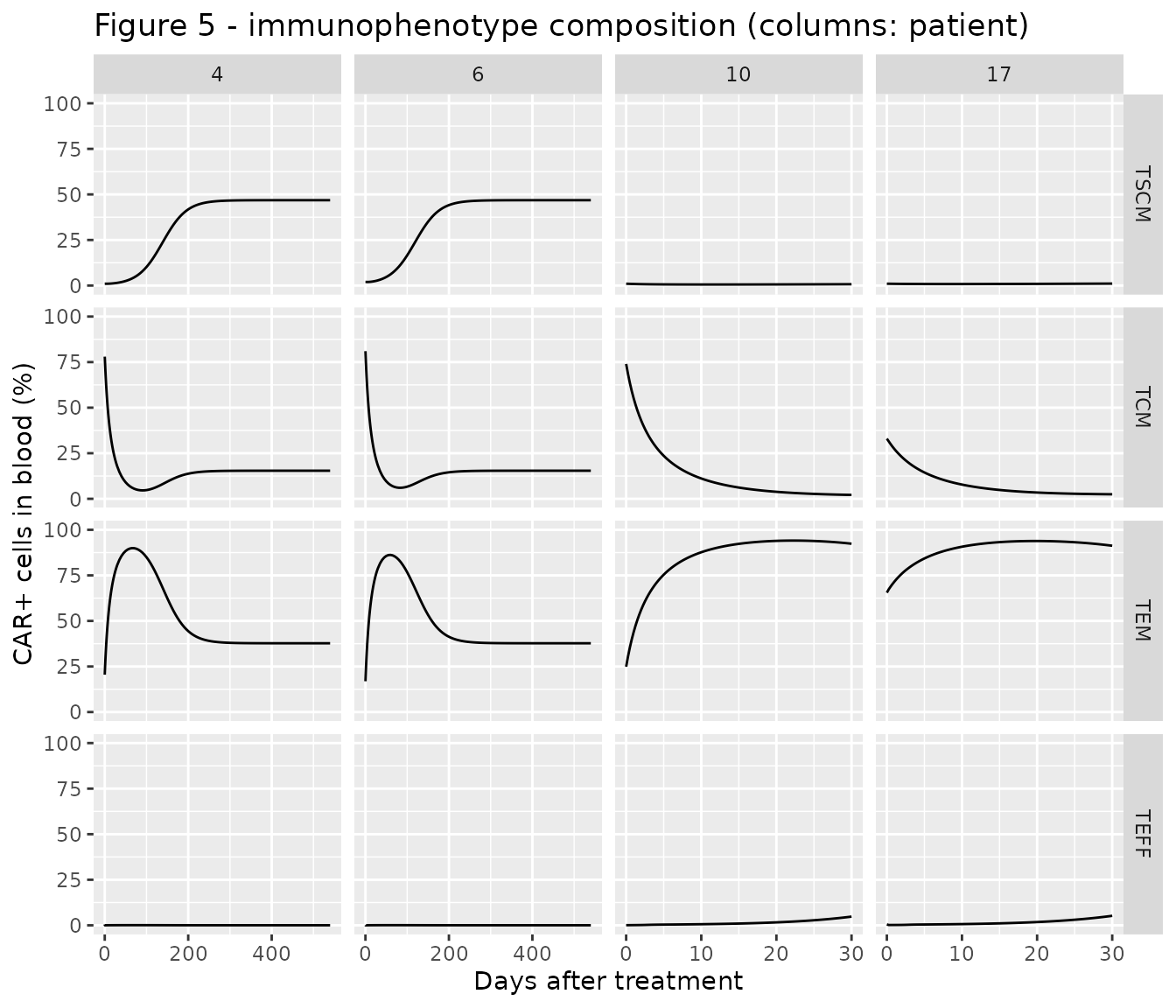
Step 3: immunophenotypes and polyclonality (Figure 5)
Each patient’s product composition (percent TSCM / TCM / TEM / TEFF
before infusion) was read by the maintainers from the time-zero points
of Figure 5; each phenotype is dosed as dose x percentage
into its CD8+ and CD4+ blood compartments, and f() applies
the 38% / 54% subset fractions. Patients 4 and 6 had a highly polyclonal
product. Their curves are shown to day 540, by which time every
phenotype percentage has reached its plateau (Figure 5 follows them to
day 720-1080); see Long-horizon simulations below for why.
immuno <- rxode2::zeroRe(uis$Salem_2023_CART_CAT19_immunophenotype_qsp)
#> Warning: No sigma parameters in the model

pts <- data.frame(
  patient = c("4", "6", "10", "17"),
  poly = c(1, 1, 0, 0),
  tscm = c(1, 2, 1, 1),
  tcm = c(78, 81, 74, 33),
  tem = c(20.5, 16.9, 24.9, 65.5),
  teff = c(0.5, 0.1, 0.1, 0.5),
  t_end = c(540, 540, 30, 30)
)

immuno_events <- function(p) {
  pct <- c(tscm = p$tscm, tcm = p$tcm, tem = p$tem, teff = p$teff)
  d <- dplyr::bind_rows(lapply(names(pct), function(ph) {
    data.frame(
      time = 0, amt = dose_cat19 * pct[[ph]] / 100, evid = 1,
      cmt = paste0(ph, c("_cd8_pb", "_cd4_pb"))
    )
  }))
  tt <- sort(unique(c(seq(0, 30, by = 0.25), seq(30, p$t_end, by = 5))))
  obs <- data.frame(time = tt, amt = 0, evid = 0, cmt = "tscm_cd8_pb")
  d <- dplyr::bind_rows(d, obs)
  d$id <- 1L
  d$WT <- wt
  d$POLYCLONALITY_HIGH <- p$poly
  d
}

sim_immuno <- dplyr::bind_rows(lapply(seq_len(nrow(pts)), function(i) {
  s <- as.data.frame(rxode2::rxSolve(immuno, immuno_events(pts[i, ]),
    atol = 1e-10, rtol = 1e-8
  ))
  s$patient <- pts$patient[i]
  s
}))
#> ℹ omega/sigma items treated as zero: 'etalkexp_max_cd8', 'etalrm1', 'etalrm2', 'etalrm3', 'etalkel_m', 'etalk12', 'etalk21'
#> ℹ omega/sigma items treated as zero: 'etalkexp_max_cd8', 'etalrm1', 'etalrm2', 'etalrm3', 'etalkel_m', 'etalk12', 'etalk21'
#> ℹ omega/sigma items treated as zero: 'etalkexp_max_cd8', 'etalrm1', 'etalrm2', 'etalrm3', 'etalkel_m', 'etalk12', 'etalk21'
#> ℹ omega/sigma items treated as zero: 'etalkexp_max_cd8', 'etalrm1', 'etalrm2', 'etalrm3', 'etalkel_m', 'etalk12', 'etalk21'
sim_immuno$patient <- factor(sim_immuno$patient, levels = pts$patient)
# Replicates Figure 5 of Salem 2023: percentage of each immunophenotype among
# blood CAR T cells.
sim_immuno |>
  dplyr::select(time, patient, TSCM = pct_tscm_pb, TCM = pct_tcm_pb, TEM = pct_tem_pb, TEFF = pct_teff_pb) |>
  tidyr::pivot_longer(c(TSCM, TCM, TEM, TEFF), names_to = "phenotype", values_to = "pct") |>
  dplyr::mutate(phenotype = factor(phenotype, levels = c("TSCM", "TCM", "TEM", "TEFF"))) |>
  ggplot(aes(time, pct)) +
  geom_line() +
  facet_grid(phenotype ~ patient, scales = "free_x") +
  coord_cartesian(ylim = c(0, 100)) +
  labs(
    x = "Days after treatment", y = "CAR+ cells in blood (%)",
    title = "Figure 5 - immunophenotype composition (columns: patient)"
  )
pick <- function(p, t, col) {
  s <- sim_immuno[sim_immuno$patient == p, ]
  s[[col]][which.min(abs(s$time - t))]
}
fig5 <- data.frame(
  check = c(
    "Patient 4 TSCM at day 365", "Patient 6 TSCM at day 365",
    "Patient 10 TCM at day 14", "Patient 17 TCM at day 14",
    "Patient 10 TEM at day 30", "Patient 17 TEM at day 14",
    "Patient 10 TSCM at day 30"
  ),
  simulated = c(
    pick("4", 365, "pct_tscm_pb"), pick("6", 365, "pct_tscm_pb"),
    pick("10", 14, "pct_tcm_pb"), pick("17", 14, "pct_tcm_pb"),
    pick("10", 30, "pct_tem_pb"), pick("17", 14, "pct_tem_pb"),
    pick("10", 30, "pct_tscm_pb")
  ),
  # Model-fitted lines of Figure 5, read by the maintainers.
  figure_5_fit = c(40, 30, 13, 2, 93, 96, 0)
)
fig5 |>
  dplyr::mutate(simulated = round(simulated, 1)) |>
  dplyr::rename(
    "Check" = check, "Simulated (%)" = simulated, "Figure 5 fit (%)" = figure_5_fit
  ) |>
knitr::kable()| Check | Simulated (%) | Figure 5 fit (%) |
|---|---|---|
| Patient 4 TSCM at day 365 | 46.8 | 40 |
| Patient 6 TSCM at day 365 | 46.8 | 30 |
| Patient 10 TCM at day 14 | 6.9 | 13 |
| Patient 17 TCM at day 14 | 5.3 | 2 |
| Patient 10 TEM at day 30 | 92.4 | 93 |
| Patient 17 TEM at day 14 | 92.9 | 96 |
| Patient 10 TSCM at day 30 | 0.7 | 0 |
# The polyclonality effect is the paper's key step-3 finding: slower
# differentiation enriches the stem-cell memory pool only in patients 4 and 6.
stopifnot(
  fig5$simulated[1] > 25, fig5$simulated[2] > 25,
  fig5$simulated[7] < 2,
  abs(fig5$simulated[5] - fig5$figure_5_fit[5]) < 10,
  abs(fig5$simulated[6] - fig5$figure_5_fit[6]) < 10
)
With the typical parameters the model reproduces the main features of Figure 5: central-memory cells convert quickly to effector memory during expansion, the low-polyclonality products (patients 10 and 17) end up almost entirely effector memory within a month, and the highly polyclonal products (patients 4 and 6) become progressively enriched in stem-cell memory cells, which plateau at about 45% of blood CAR T cells (Figure 5a fits: about 40% and 30%). The terminal-effector hump in patients 4 and 6 (Figure 5d, up to about 25% around day 100) is not reproduced: with the effector elimination rate fixed at 113 /day, blood TEFF cells stay below 1% of CAR T cells (see Assumptions and deviations).
Assumptions and deviations
- Five model files. The step-1 in vitro fit treats FMC63 and CAT19 in one Monolix run, but every estimated parameter and both binding constants are construct-specific and no random effect was estimated, so the joint fit separates exactly into two files. Steps 2 (Liso-cel, CAT19) and 3 are separate fits.
- Cell states carried as numbers. The Monolix code carries CAR T-cell pools as concentrations (cells/L) and doses “cells/L”; the packaged models carry them as cell numbers so a dose record is a number of cells. The transformation is exact (every CAR T-cell flux is a rate constant times a concentration times a fixed volume). Complexes and tumour cells stay as concentrations.
-
Dosing the CD4 / CD8 split. The total dose is given
once on the CD8+ and once on the CD4+ blood compartment, and
f()applies the product fractions (Liso-cel 50 / 50%; CAT19 38 / 54%, Table 2). In the step-2 CAT19 model the 50% random effects on PCTCD8 and PCTCD4 enter throughf(). In step 3 each immunophenotype is dosed the same way. - Memory elimination term. Appendix S1 Eqs. 7 and 10 omit the elimination of memory cells from blood, but the text (“first-order elimination rate constant (Kelm) occurs in PB compartment only for both subtypes”) and the Monolix code both include it; it is included.
-
Tumour kill flux. The kill rate
KKillMax x CplxTumor / (KC50 + CplxTumor)multiplied by the tumour concentration is written asKKillMax x Cplx x Tumor / (KC50 x Tumor + Cplx), which is identical for a non-zero tumour and gives zero (not 0/0) when the DLBCL blood tumour burden is zero. -
Pre-dose switch. The Monolix code sets tumour
growth and killing to zero for
t <= 0; with dosing at time zero this has no effect and is omitted. - Months to days. Table 2 reports the step-2 CAT19 rate constants per month. The packaged model uses the per-day values printed in the Results and the step-3 table (KmaxExpCD8 5.3, Kelm 0.013, Rm 0.000037, K12 0.11 /day), which equal the monthly values divided by 30. The Discussion quotes Rm as 0.00003 /day; the Results value 0.000037 is used.
-
Volumes. Table 2 prints the CAT19 volumes as “5 *
3070” and “1.6 * 3070”; these are 5 x 30/70 and 1.6 x 30/70 L, the adult
volumes scaled to the 30 kg weight assumed for every child. The packaged
CAT19 models scale both volumes by
WT/70(as the step-3 Monolix code does), soWT = 30reproduces the paper. - qPCR link. Liso-cel uses the published tisagenlecleucel relationship ln(copies/ug gDNA) = 7.6204 + 0.8537 ln(cells/uL) (Eq. 1; Table 2 rounds to 7.62 / 0.85). The CAT19 model uses its own estimates (7.26 / 0.74) for both blood and bone marrow (Figure 4 fits qPCR in both). Table 2 lists no qPCR link for step 3; the step-2 CAT19 values are used because the paper states that the step-3 CK parameters were carried over from step 2.
-
Step 3: Table 2 and Appendix S1 over the Appendix S2
code. The step-3 Monolix code in Appendix S2 is an earlier
iteration: it uses a single
rmfor every blood transition, KC50 4.05, an initial bone-marrow tumour burden of 7.8E10 cells/L, a qPCR link of 6.42 / 0.823 and no polyclonality effect. The packaged model follows Table 2 and Appendix S1 Eqs. 43-66 (separate Rm1-Rm3, KC50 0.28, 1.06E11 cells/L, polyclonality on Rm1-Rm3). The Appendix S1 equations are written for one subset “applying similarly for both CD4 and CD8 subsets”; each subset keeps its own complexes, as in step 2 and the code. - KmaxExpCD4 in step 3. Table 2 prints “KmaxExpCD8/1.12 = 2.9”, but 3.44 / 1.12 = 3.07; the ratio form is used.
-
Polyclonality covariate.
POLYCLONALITY_HIGH(1 = high clonal diversity of the infusion product) multiplies Rm1, Rm2 and Rm3 by 0.08, 0.21 and 0.19, the reductions of about 92%, 79% and 81% quoted in the Discussion. - Terminal-effector fraction. With Kele fixed at 113 /day, blood TEFF cells are cleared within hours and stay below 1% of blood CAR T cells, so the model cannot produce the 10-25% TEFF fractions of the Figure 5d fits for patients 4 and 6. The maintainers did not alter Kele; the discrepancy suggests the published fit used a different TEFF elimination than Table 2 reports.
-
Long-horizon simulations. Once the CAR T cells
eradicate the tumour (for CAT19, by about day 60, to around 1E-20
cells/L), the two tumour states sit at the solver’s absolute-tolerance
noise. The exponential growth term amplifies that noise (by e^(0.065 t)
for the 10.7-day CAT19 doubling time), so a solution can drift negative,
or seed a spurious relapse, roughly 1.5-2 years after eradication.
Exactly when depends on the tolerances. With the step-3 model, patient 4
to day 1080 failed to solve at some tolerance settings and drifted to a
tumour concentration of -2E7 cells/L by day 800 at the default ones.
Over the first 540 days the immunophenotype percentages agree to four
significant figures across
atol1E-8 to 1E-12. This article therefore stops the CAT19 simulations at 365 days (step 2) and 540 days (step 3). The behaviour belongs to the published equations, which have no floor on the tumour states, and the models are left unchanged. - Uncontrolled tumour growth. The tumour model has no carrying capacity either. A virtual child whose sampled random effects leave the tumour uncontrolled (the large omegas on Rm, K12 and K21 allow this) sees blood tumour grow to around 1E19 cells/L within a year, and at that scale the solver cannot follow the CAR-CD19 binding. These few subjects return as NA and the Figure 4 cohort drops them, reporting how many.
- Random effects. Monolix omegas are standard deviations of log-normal random effects; the models encode their squares as variances. In the Liso-cel model the fixed 50% random effect on KKillMax represents the heterogeneity between the ALL and DLBCL summary profiles, so the per-panel Figure 2b fits (each with its own KKillMax) differ from the typical-value curves shown here.
-
No residual-error model. The paper describes the
error models (M3 censoring below the LLOQ in step 2; an additive
logit-normal error for the step-3 percentages) but does not report their
estimates, so none is encoded. Use
rxode2::zeroRe()for typical-value trajectories. - Digitised targets. The Figure 1b, 2b1, 4 and 5 comparison values and the step-3 product compositions were read from the published figures by the maintainers; Appendix S1 Table S1 values are printed.
- Errata. No erratum or correction was found for this article (EuropePMC search, October 2026).