Sunitinib and SU012662 in children (Wang 2021)
Source:vignettes/articles/Wang_2021_sunitinib.Rmd
Wang_2021_sunitinib.RmdModel and source
- Citation: Wang E, DuBois SG, Wetmore C, Verschuur AC, Khosravan R (2021). Population Pharmacokinetics of Sunitinib and its Active Metabolite SU012662 in Pediatric Patients with Gastrointestinal Stromal Tumors or Other Solid Tumors. Eur J Drug Metab Pharmacokinet 46(3):343-352. doi:10.1007/s13318-021-00671-7.
- Parent model: Two-compartment population PK model for oral sunitinib (parent drug) in 65 children, adolescents and young adults (3-21 years) with gastrointestinal stromal tumors or other solid / CNS tumors (Wang 2021). First-order absorption with a lag time; apparent clearance CL/F and central volume Vc/F scale with body surface area as power functions normalised to 1.44 m^2. Exponential IIV on CL/F, Vc/F and ka; proportional residual error. The active metabolite SU012662 was fitted as a separate model and ships as Wang_2021_sunitinib_su12662.
- Metabolite model: Two-compartment population PK model for SU012662 (N-desethyl sunitinib, the primary active metabolite) after oral sunitinib in 65 children, adolescents and young adults (3-21 years) with gastrointestinal stromal tumors or other solid / CNS tumors (Wang 2021). Fitted separately from the parent: the sunitinib dose enters a first-order absorption depot with a lag time, with a fixed 21% of the sunitinib dose assumed converted to SU012662, so the metabolite clearances and volumes are apparent values relative to that fraction and the unknown oral bioavailability. CL/F and Vc/F scale with body surface area as power functions normalised to 1.44 m^2. Exponential IIV on CL/F, Vc/F and ka; proportional residual error. The parent model ships as Wang_2021_sunitinib.
- Article: https://doi.org/10.1007/s13318-021-00671-7
Wang 2021 is the first population PK analysis of sunitinib in children. The authors fitted two separate models – one to the sunitinib (parent) concentrations and one to the SU012662 (N-desethyl sunitinib) concentrations – “as have been used previously in adults … and to enable direct comparison between adult and pediatric data” (Methods 2.3). Both are two-compartment models with first-order absorption and a lag time, driven by the oral sunitinib dose. For the metabolite model the authors assumed that 21% of the sunitinib dose is converted to SU012662 (Results 3.3). Body surface area (BSA) was the only covariate retained in either model, on CL/F and Vc/F.
The two models are shipped as two files that share this article:
Wang_2021_sunitinib (observation Cc,
sunitinib) and Wang_2021_sunitinib_su12662 (observation
Cc_su12662, SU012662). They are not coupled: each takes the
sunitinib dose into its own depot.
# readModelDb() returns the model function; resolve each to its rxUi once.
mod_p <- rxode2::rxode(readModelDb("Wang_2021_sunitinib"))
#> ℹ parameter labels from comments will be replaced by 'label()'
mod_m <- rxode2::rxode(readModelDb("Wang_2021_sunitinib_su12662"))
#> ℹ parameter labels from comments will be replaced by 'label()'
mod_p$state
#> [1] "depot"       "central"     "peripheral1"
mod_m$state
#> [1] "depot"               "central_su12662"     "peripheral1_su12662"
Population
Data were pooled from three studies of oral sunitinib in pediatric patients (Table 1): ADVL0612 (phase 1, 35 evaluable patients with refractory solid tumors, mostly CNS), ACNS1021 (phase 2, 24 patients with high-grade glioma or ependymoma) and A6181196 (phase 1/2, 6 patients with gastrointestinal stromal tumor, GIST). All three used schedule 4/2 (4 weeks on, 2 weeks off) at a starting dose of 15 or 20 mg/m^2 once daily, given as an intact capsule or as capsule contents sprinkled on yogurt or applesauce.
The 65 patients were 3-21 years old (median 13), 50.8% female, 4 Asian, 58 non-Asian and 3 of unknown race; median body weight was 49.1 kg (16.2-100) and median BSA 1.4 m^2 (0.7-2.1) (Table 2). The dataset held 439 sunitinib and 417 SU012662 post-baseline observations.
The same information is available programmatically via
readModelDb("Wang_2021_sunitinib")()$population.
Source trace
Every ini() entry in the two model files carries an
in-file comment pointing at its origin. They are collected here for
review. Table 3 is the final-model parameter table; Results 3.2 and 3.3
print the final covariate equations.
| Equation / parameter | Sunitinib | SU012662 | Source location |
|---|---|---|---|
lcl / lcl_su12662 (CL/F at BSA 1.44
m^2) |
24.0 L/h | 11.1 L/h | Table 3, theta1 |
lvc / lvc_su12662 (Vc/F at BSA 1.44
m^2) |
1030 L | 1060 L | Table 3, theta2 |
lka / lka_su12662 (ka) |
0.37 1/h | 0.28 1/h | Table 3, theta3 |
ltlag / ltlag_su12662 (lag time) |
0.76 h | 0.64 h | Table 3, theta4 |
lvp / lvp_su12662 (Vp/F) |
81.3 L | 63.1 L | Table 3, theta5 |
lq / lq_su12662 (Q/F) |
0.39 L/h | 6.7 L/h | Table 3, theta6 |
e_bsa_cl / e_bsa_cl_su12662
|
0.733 | 0.87 | Results 3.2 / 3.3 printed equations; Table 3 theta9 (0.73 / 0.87) |
e_bsa_vc / e_bsa_vc_su12662
|
1.46 | 1.61 | Results 3.2 / 3.3 printed equations; Table 3 theta8 |
etalcl / etalcl_su12662
|
0.1034 (33%) | 0.1770 (44%) | Table 3 omega CL/F, log(1 + CV^2)
|
etalvc / etalvc_su12662
|
0.06204 (25.3%) | 0.1625 (42%) | Table 3 omega Vc/F, log(1 + CV^2)
|
etalka / etalka_su12662
|
0.7271 (103.4%) | 0.6502 (95.7%) | Table 3 omega ka, log(1 + CV^2)
|
propSd / propSd_su12662
|
0.322 | 0.26 | Table 3, sigma (theta7) |
fm (fraction of dose converted) |
n/a | fixed(0.21) |
Results 3.3, “a conversion of 21% sunitinib to SU012662 was assumed” |
BSA covariate form (BSA/1.44)^theta
|
n/a | n/a | Results 3.2 and 3.3 |
| Two-compartment, first-order absorption with lag | n/a | n/a | Methods 2.3; Results 3.2 and 3.3 |
Exponential IIV theta_i = theta * exp(eta_i), no omega
block |
n/a | n/a | Methods 2.3; Results 3.2 and 3.3 |
Structural checks
These checks use a single typical subject per BSA with the random effects set to zero, so they are deterministic and hold at any solver-thread count.
# One subject per row of `subj` (columns id, BSA, dose_mg, label), dosed once
# daily for `n_days` days. The observation grid is supplied by the caller.
# Observation rows sit on an ODE state (`central` / `central_su12662`), never on
# the algebraic observable.
make_daily_events <- function(subj, n_days, obs_times, obs_cmt) {
  dose <- subj |>
    dplyr::mutate(
      time = 0, amt = dose_mg, cmt = "depot", evid = 1L,
      ii = 24, addl = n_days - 1L
    )
  obs <- subj |>
    tidyr::crossing(time = obs_times) |>
    dplyr::mutate(amt = NA_real_, cmt = obs_cmt, evid = 0L, ii = 0, addl = 0L)
  dplyr::bind_rows(dose, obs) |>
    dplyr::arrange(id, time, dplyr::desc(evid)) |>
    as.data.frame()
}

# Linear trapezoid over one subject's profile.
trap_auc <- function(time, conc) {
  sum(diff(time) * (utils::head(conc, -1) + utils::tail(conc, -1)) / 2)
}

# rxode2 warns that a multi-subject solve has no omega once the random effects
# are zeroed; that is the intent here, so only that one warning is muffled.
muffle_no_omega <- function(w) {
  if (grepl("without 'omega'", conditionMessage(w), fixed = TRUE)) {
    invokeRestart("muffleWarning")
  }
}

solve_typical <- function(mod, events, keep) {
  withCallingHandlers(
    rxode2::rxSolve(
      rxode2::zeroRe(mod), events,
      keep = keep, returnType = "data.frame",
      rtol = 1e-10, atol = 1e-12, maxsteps = 1e6
    ),
    warning = muffle_no_omega
  )
}
Covariate equations
The individual CL/F and Vc/F computed inside each model are compared with the paper’s printed final equations, transcribed independently here.
bsa_grid <- tibble::tibble(id = 1:6, BSA = c(0.5, 0.7, 1.1, 1.44, 1.6, 2.1), dose_mg = 20, label = "grid")
ev_p <- make_daily_events(bsa_grid, 1L, c(1, 2), "central")
ev_m <- make_daily_events(bsa_grid, 1L, c(1, 2), "central_su12662")
cov_p <- solve_typical(mod_p, ev_p, keep = "BSA") |> dplyr::distinct(id, BSA, cl, vc)
#> ℹ omega/sigma items treated as zero: 'etalcl', 'etalvc', 'etalka'
cov_m <- solve_typical(mod_m, ev_m, keep = "BSA") |> dplyr::distinct(id, BSA, cl_su12662, vc_su12662)
#> ℹ omega/sigma items treated as zero: 'etalcl_su12662', 'etalvc_su12662', 'etalka_su12662'

cov_chk <- dplyr::inner_join(cov_p, cov_m, by = c("id", "BSA")) |>
  dplyr::mutate(
    paper_cl = 24 * (BSA / 1.44)^0.733,
    paper_vc = 1030 * (BSA / 1.44)^1.46,
    paper_cl_m = 11.1 * (BSA / 1.44)^0.87,
    paper_vc_m = 1060 * (BSA / 1.44)^1.61
  )
stopifnot(nrow(cov_chk) == nrow(bsa_grid))
stopifnot(
  max(abs(cov_chk$cl / cov_chk$paper_cl - 1)) < 1e-10,
  max(abs(cov_chk$vc / cov_chk$paper_vc - 1)) < 1e-10,
  max(abs(cov_chk$cl_su12662 / cov_chk$paper_cl_m - 1)) < 1e-10,
  max(abs(cov_chk$vc_su12662 / cov_chk$paper_vc_m - 1)) < 1e-10
)

cov_chk |>
  dplyr::transmute(
    "BSA (m^2)" = BSA,
    "Sunitinib CL/F (L/h)" = signif(cl, 4),
    "Sunitinib Vc/F (L)" = signif(vc, 4),
    "SU012662 CL/F (L/h)" = signif(cl_su12662, 4),
    "SU012662 Vc/F (L)" = signif(vc_su12662, 4)
  ) |>
knitr::kable(caption = "Typical apparent clearance and central volume by BSA (reproduce the printed equations of Results 3.2 and 3.3).")| BSA (m^2) | Sunitinib CL/F (L/h) | Sunitinib Vc/F (L) | SU012662 CL/F (L/h) | SU012662 Vc/F (L) |
|---|---|---|---|---|
| 0.50 | 11.05 | 219.8 | 4.422 | 193.1 |
| 0.70 | 14.14 | 359.3 | 5.926 | 331.9 |
| 1.10 | 19.70 | 695.1 | 8.781 | 687.0 |
| 1.44 | 24.00 | 1030.0 | 11.100 | 1060.0 |
| 1.60 | 25.93 | 1201.0 | 12.170 | 1256.0 |
| 2.10 | 31.65 | 1787.0 | 15.410 | 1946.0 |
Reproducing the paper’s dose-finding calculation
Section 3.4 derives, from the final models, the sunitinib dose that gives a typical child the same steady-state 24-h AUC as an adult with GIST receiving 50 mg/day: 1233 ng.h/mL for sunitinib and 551 ng.h/mL for SU012662. The paper reports the answer for three age groups at their median BSA. The chunk below solves each model to steady state on once-daily dosing at 20 mg/m^2, measures AUC over the last dosing interval, and scales to the dose that would hit the adult reference (the models are linear, so AUC is proportional to dose).
TAU_START <- 59 * 24
tau_grid <- seq(TAU_START, TAU_START + 24, by = 0.05)

age_groups <- tibble::tibble(
  id = 1:3,
  label = c("2-5 years", "6-11 years", "12-17 years"),
  BSA = c(0.69, 1.1, 1.6), # median BSA stated in Section 3.4
  dose_mg = 20 * c(0.69, 1.1, 1.6)
)

ss_p <- solve_typical(mod_p, make_daily_events(age_groups, 60L, tau_grid, "central"), keep = c("label", "BSA"))
#> ℹ omega/sigma items treated as zero: 'etalcl', 'etalvc', 'etalka'
ss_m <- solve_typical(mod_m, make_daily_events(age_groups, 60L, tau_grid, "central_su12662"), keep = c("label", "BSA"))
#> ℹ omega/sigma items treated as zero: 'etalcl_su12662', 'etalvc_su12662', 'etalka_su12662'

auc_p <- ss_p |>
  dplyr::group_by(id, label, BSA) |>
  dplyr::summarise(auc = trap_auc(time, Cc), cl = cl[1], .groups = "drop")
auc_m <- ss_m |>
  dplyr::group_by(id, label, BSA) |>
  dplyr::summarise(auc = trap_auc(time, Cc_su12662), cl = cl_su12662[1], .groups = "drop")

# Steady-state mass balance: CL/F * AUCtau recovers the dose delivered to each
# model's depot (all of it for sunitinib, fm = 21% of it for SU012662).
# CL (L/h) * AUC (ng.h/mL = ug.h/L) / 1000 = mg.
mb_p <- auc_p$cl * auc_p$auc / 1000 / age_groups$dose_mg
mb_m <- auc_m$cl * auc_m$auc / 1000 / (0.21 * age_groups$dose_mg)
stopifnot(max(abs(mb_p - 1)) < 1e-3, max(abs(mb_m - 1)) < 1e-3)

dose_tbl <- tibble::tibble(
  "Age group" = age_groups$label,
  "Median BSA (m^2)" = age_groups$BSA,
  "Sunitinib: model dose (mg/m^2)" = 20 * 1233 / auc_p$auc,
  "Sunitinib: paper (mg/m^2)" = c(25, 22, 20),
  "SU012662: model dose (mg/m^2)" = 20 * 551 / auc_m$auc,
  "SU012662: paper (mg/m^2)" = c(22, 21, 20)
)

# The paper reports the doses rounded to whole mg/m^2; all six must round to
# the printed value. Each model value sits 0.24-0.49 mg/m^2 (1-2.5%) from a
# rounding boundary, far beyond the numerical error of the solve, while an
# error of a few percent in a clearance, an exponent, the 1.44 m^2 centre or
# fm moves at least one of them across its boundary.
stopifnot(
  all(round(dose_tbl[["Sunitinib: model dose (mg/m^2)"]]) == dose_tbl[["Sunitinib: paper (mg/m^2)"]]),
  all(round(dose_tbl[["SU012662: model dose (mg/m^2)"]]) == dose_tbl[["SU012662: paper (mg/m^2)"]])
)

dose_tbl |>
  dplyr::mutate(dplyr::across(dplyr::contains("model dose"), \(x) round(x, 2))) |>
knitr::kable(caption = "Sunitinib dose giving the adult reference steady-state AUC (1233 / 551 ng.h/mL), by age group. Reproduces Section 3.4 of Wang 2021.")| Age group | Median BSA (m^2) | Sunitinib: model dose (mg/m^2) | Sunitinib: paper (mg/m^2) | SU012662: model dose (mg/m^2) | SU012662: paper (mg/m^2) |
|---|---|---|---|---|---|
| 2-5 years | 0.69 | 25.01 | 25 | 22.26 | 22 |
| 6-11 years | 1.10 | 22.08 | 22 | 20.95 | 21 |
| 12-17 years | 1.60 | 19.98 | 20 | 19.95 | 20 |
Every one of the six doses reported in Section 3.4 is reproduced. This also settles two points the paper does not state explicitly: the 21% conversion is applied on a mass basis (no molecular-weight correction), and the reference BSA of 1.44 m^2 is the normalising constant of both covariate models.
BSA-tiered doses
Section 3.4 also proposes a flat-dose tiering by BSA: 12.5 mg (BSA <= 0.7 m^2), 25 mg (0.8-1.5 m^2), 37.5 mg (1.6-2.4 m^2) and 50 mg (>= 2.5 m^2), each described as giving an AUC “approximately similar” to the adult reference. The typical-subject AUC ratio at each tier boundary is shown below.
tiers <- tibble::tibble(
  id = 1:6,
  BSA = c(0.7, 0.8, 1.5, 1.6, 2.4, 2.5),
  dose_mg = c(12.5, 25, 25, 37.5, 37.5, 50),
  label = "tier"
)
tier_p <- solve_typical(mod_p, make_daily_events(tiers, 60L, tau_grid, "central"), keep = "BSA") |>
  dplyr::group_by(id, BSA) |>
  dplyr::summarise(ratio_p = trap_auc(time, Cc) / 1233, .groups = "drop")
#> ℹ omega/sigma items treated as zero: 'etalcl', 'etalvc', 'etalka'
tier_m <- solve_typical(mod_m, make_daily_events(tiers, 60L, tau_grid, "central_su12662"), keep = "BSA") |>
  dplyr::group_by(id, BSA) |>
  dplyr::summarise(ratio_m = trap_auc(time, Cc_su12662) / 551, .groups = "drop")
#> ℹ omega/sigma items treated as zero: 'etalcl_su12662', 'etalvc_su12662', 'etalka_su12662'
tier_tbl <- tiers |>
  dplyr::inner_join(tier_p, by = c("id", "BSA")) |>
  dplyr::inner_join(tier_m, by = c("id", "BSA"))

# Deterministic. Realised ratios span 0.72-1.30 (sunitinib) and 0.80-1.43
# (SU012662); the lowest sits at the 0.7 m^2 top of the 12.5 mg tier and the
# highest at the 0.8 m^2 bottom of the 25 mg tier, where the flat dose doubles.
stopifnot(nrow(tier_tbl) == 6L)
stopifnot(all(tier_tbl$ratio_p > 0.65 & tier_tbl$ratio_p < 1.5))
stopifnot(all(tier_tbl$ratio_m > 0.65 & tier_tbl$ratio_m < 1.5))

tier_tbl |>
  dplyr::transmute(
    "BSA (m^2)" = BSA, "Dose (mg)" = dose_mg,
    "Sunitinib AUC / 1233" = round(ratio_p, 2),
    "SU012662 AUC / 551" = round(ratio_m, 2)
  ) |>
knitr::kable(caption = "Typical steady-state AUC relative to the adult reference at the boundaries of the BSA-tiered doses of Section 3.4.")| BSA (m^2) | Dose (mg) | Sunitinib AUC / 1233 | SU012662 AUC / 551 |
|---|---|---|---|
| 0.7 | 12.5 | 0.72 | 0.80 |
| 0.8 | 25.0 | 1.30 | 1.43 |
| 1.5 | 25.0 | 0.82 | 0.83 |
| 1.6 | 37.5 | 1.17 | 1.17 |
| 2.4 | 37.5 | 0.87 | 0.83 |
| 2.5 | 50.0 | 1.13 | 1.06 |
The ratios bracket 1 and span roughly 0.7-1.4, i.e. somewhat wider than the 0.75-1.25 band the paper uses for its per-m^2 dose (Figure 3); the paper itself only calls the tiered doses “approximately similar”.
Virtual cohort
Original observed data are not publicly available. The cohort reproduces the age-group composition of Table 2 (6 / 20 / 33 / 6 patients aged 2-5 / 6-11 / 12-17 / 18-21 years) at twice the size, 130 subjects in total. Within each age group BSA is drawn log-normally around the group median and redrawn until it falls inside the group’s reported range (a band limit is a definition of the group, so values are never clipped onto its edges).
# set.seed() seeds R's RNG for the BSA draw only; rxode2's between-subject
# draws differ across solver-thread counts, so every assertion below is written
# to hold for any cohort the model can produce.
set.seed(20210414)

draw_bsa <- function(n, med, lo, hi, sdlog = 0.15) {
  out <- numeric(0)
  while (length(out) < n) {
    x <- exp(rnorm(n, log(med), sdlog))
    out <- c(out, x[x >= lo & x <= hi])
  }
  out[seq_len(n)]
}

groups <- tibble::tribble(
  ~age_group, ~n, ~med, ~lo, ~hi,
  "2-5 years", 12L, 0.7, 0.65, 1.0,
  "6-11 years", 40L, 1.1, 0.7, 1.5,
  "12-17 years", 66L, 1.6, 1.3, 2.1,
  "18-21 years", 12L, 1.9, 1.6, 1.95
)

cohort <- do.call(rbind, lapply(seq_len(nrow(groups)), function(i) {
  data.frame(
    age_group = groups$age_group[i],
    BSA = draw_bsa(groups$n[i], groups$med[i], groups$lo[i], groups$hi[i])
  )
}))
cohort$id <- seq_len(nrow(cohort))
cohort$age_group <- factor(cohort$age_group, levels = groups$age_group)
stopifnot(nrow(cohort) == 130L, !anyDuplicated(cohort$id))
stopifnot(all(cohort$BSA >= 0.65 & cohort$BSA <= 2.1))

# Schedule 4/2 at 15 mg/m^2 (the dose of the Figure 2 VPCs): 28 daily doses,
# 14 days off, three cycles (about 3000 h, the span of Figure 2c-d).
CYCLE_H <- 42 * 24
make_schedule42 <- function(cohort, obs_times, obs_cmt) {
  dose <- cohort |>
    tidyr::crossing(cycle = 0:2) |>
    dplyr::mutate(
      time = cycle * CYCLE_H, amt = 15 * BSA, cmt = "depot", evid = 1L,
      ii = 24, addl = 27L
    ) |>
    dplyr::select(-cycle)
  obs <- cohort |>
    tidyr::crossing(time = obs_times) |>
    dplyr::mutate(amt = NA_real_, cmt = obs_cmt, evid = 0L, ii = 0, addl = 0L)
  dplyr::bind_rows(dose, obs) |>
    dplyr::arrange(id, time, dplyr::desc(evid)) |>
    as.data.frame()
}

OBS <- sort(unique(c(seq(0, 24, by = 0.5), seq(24, 3 * CYCLE_H, by = 12))))
ev_cohort_p <- make_schedule42(cohort, OBS, "central")
ev_cohort_m <- make_schedule42(cohort, OBS, "central_su12662")
stopifnot(!anyDuplicated(unique(ev_cohort_p[, c("id", "time", "evid")])))
Simulation
rxode2::rxSetSeed(2021)
sim_p <- rxode2::rxSolve(mod_p, ev_cohort_p,
  keep = c("age_group", "BSA"), returnType = "data.frame", maxsteps = 1e6
)
sim_m <- rxode2::rxSolve(mod_m, ev_cohort_m,
  keep = c("age_group", "BSA"), returnType = "data.frame", maxsteps = 1e6
)
stopifnot(!anyNA(sim_p$Cc), !anyNA(sim_m$Cc_su12662))
stopifnot(all(sim_p$Cc >= -1e-6 * max(sim_p$Cc)), all(sim_m$Cc_su12662 >= -1e-6 * max(sim_m$Cc_su12662)))

sim <- dplyr::bind_rows(
  sim_p |> dplyr::transmute(id, time, age_group, BSA, analyte = "Sunitinib", conc = Cc),
  sim_m |> dplyr::transmute(id, time, age_group, BSA, analyte = "SU012662", conc = Cc_su12662)
) |>
  dplyr::mutate(analyte = factor(analyte, levels = c("Sunitinib", "SU012662")))
Replicate published figures
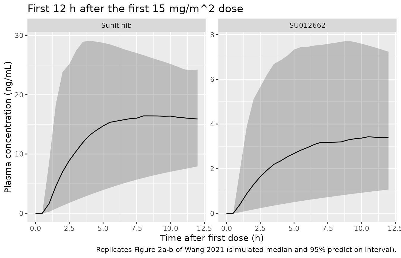
Figure 2 of Wang 2021 shows the visual predictive checks of the final models at 15 mg/m^2 on schedule 4/2: panels a-b over the first 12 h after the first dose and panels c-d over about 3000 h. The panels below show the simulated median and 2.5th / 97.5th percentiles; the observed data are not available.
vpc_summary <- function(d) {
  d |>
    dplyr::group_by(analyte, time) |>
    dplyr::summarise(
      lo = quantile(conc, 0.025), med = median(conc), hi = quantile(conc, 0.975),
      .groups = "drop"
    )
}

sim |>
  dplyr::filter(time <= 12) |>
  vpc_summary() |>
  ggplot(aes(time, med)) +
  geom_ribbon(aes(ymin = lo, ymax = hi), alpha = 0.25) +
  geom_line() +
  facet_wrap(~analyte, scales = "free_y") +
  labs(
    x = "Time after first dose (h)", y = "Plasma concentration (ng/mL)",
    title = "First 12 h after the first 15 mg/m^2 dose",
    caption = "Replicates Figure 2a-b of Wang 2021 (simulated median and 95% prediction interval)."
  )
sim |>
  dplyr::filter(time >= 24) |>
  vpc_summary() |>
  ggplot(aes(time, med)) +
  geom_ribbon(aes(ymin = lo, ymax = hi), alpha = 0.25) +
  geom_line() +
  facet_wrap(~analyte, scales = "free_y", ncol = 1) +
  labs(
    x = "Time after first dose (h)", y = "Plasma concentration (ng/mL)",
    title = "Three cycles of schedule 4/2 at 15 mg/m^2",
    caption = "Replicates Figure 2c-d of Wang 2021 (simulated median and 95% prediction interval, 12-h grid)."
  )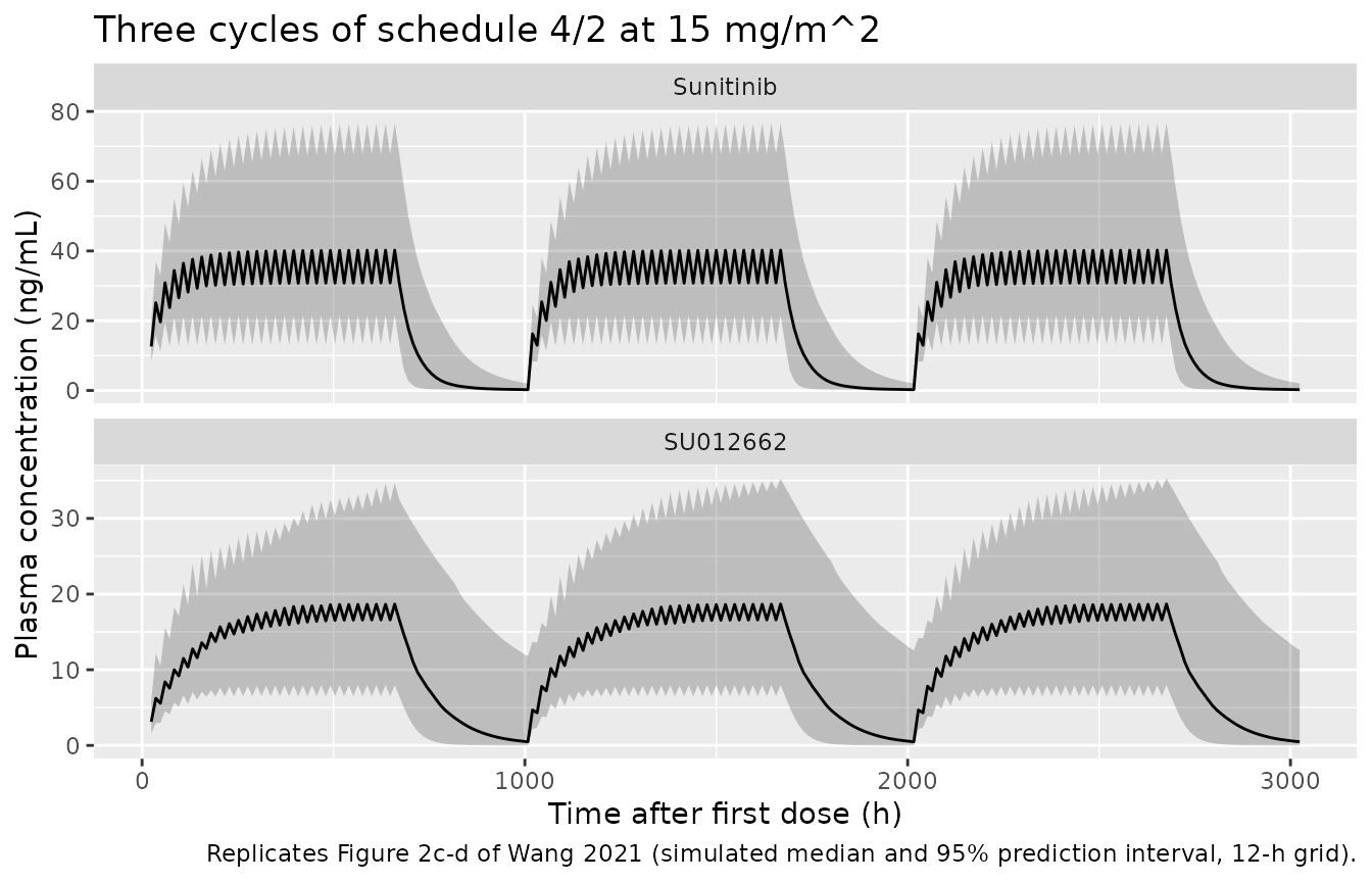
The lag times (0.76 h and 0.64 h) are visible as the flat start of the first-dose profiles, and SU012662 accumulates more slowly and to a lower level than sunitinib over each 4-week on-period, consistent with the adult behaviour described in the paper’s introduction.
PKNCA validation
NCA is run per age group and analyte over the first dosing interval (day 1) and over the last dosing interval of the first on-period (day 28).
DAY28 <- c(27 * 24, 28 * 24)
sim_nca <- sim |>
  dplyr::filter(!is.na(conc), time <= DAY28[2]) |>
  dplyr::mutate(conc = pmax(conc, 0)) |>
  dplyr::rename(Cc = conc)

# Oral dosing: the pre-dose concentration at t = 0 is zero.
sim_nca <- dplyr::bind_rows(
  sim_nca,
  sim_nca |> dplyr::distinct(id, age_group, analyte, BSA) |> dplyr::mutate(time = 0, Cc = 0)
) |>
  dplyr::distinct(id, age_group, analyte, time, .keep_all = TRUE) |>
  dplyr::arrange(id, age_group, analyte, time)

dose_df <- ev_cohort_p |>
  dplyr::filter(evid == 1, time == 0) |>
  dplyr::select(id, time, amt, age_group) |>
  tidyr::crossing(analyte = c("Sunitinib", "SU012662"))

conc_obj <- PKNCA::PKNCAconc(
  as.data.frame(sim_nca), Cc ~ time | age_group + analyte + id,
  concu = "ng/mL", timeu = "h"
)
dose_obj <- PKNCA::PKNCAdose(
  as.data.frame(dose_df), amt ~ time | age_group + analyte + id,
  doseu = "mg"
)
intervals <- data.frame(
  start = c(0, DAY28[1]), end = c(24, DAY28[2]),
  cmax = TRUE, tmax = TRUE, auclast = TRUE
)
nca_res <- PKNCA::pk.nca(PKNCA::PKNCAdata(conc_obj, dose_obj, intervals = intervals))
nca_tbl <- as.data.frame(nca_res$result)
stopifnot(nrow(nca_tbl) > 0)

nca_tbl |>
  dplyr::filter(PPTESTCD %in% c("cmax", "auclast")) |>
  dplyr::mutate(interval = ifelse(start == 0, "Day 1", "Day 28")) |>
  dplyr::group_by(analyte, interval, age_group, PPTESTCD) |>
  dplyr::summarise(median = signif(median(PPORRES), 3), .groups = "drop") |>
  tidyr::pivot_wider(names_from = PPTESTCD, values_from = median) |>
  dplyr::arrange(analyte, interval, age_group) |>
  dplyr::rename(
    Analyte = analyte, Interval = interval, "Age group" = age_group,
    "Median Cmax (ng/mL)" = cmax, "Median AUC0-24 (ng.h/mL)" = auclast
  ) |>
knitr::kable(caption = "Simulated NCA at 15 mg/m^2 once daily by age group (median over subjects).")| Analyte | Interval | Age group | Median AUC0-24 (ng.h/mL) | Median Cmax (ng/mL) |
|---|---|---|---|---|
| SU012662 | Day 1 | 2-5 years | 99.6 | 5.05 |
| SU012662 | Day 1 | 6-11 years | 78.0 | 4.01 |
| SU012662 | Day 1 | 12-17 years | 61.2 | 3.12 |
| SU012662 | Day 1 | 18-21 years | 76.6 | 3.82 |
| SU012662 | Day 28 | 2-5 years | 498.0 | 21.90 |
| SU012662 | Day 28 | 6-11 years | 420.0 | 18.70 |
| SU012662 | Day 28 | 12-17 years | 421.0 | 18.20 |
| SU012662 | Day 28 | 18-21 years | 413.0 | 18.00 |
| Sunitinib | Day 1 | 2-5 years | 408.0 | 24.20 |
| Sunitinib | Day 1 | 6-11 years | 367.0 | 19.90 |
| Sunitinib | Day 1 | 12-17 years | 307.0 | 15.90 |
| Sunitinib | Day 1 | 18-21 years | 261.0 | 13.50 |
| Sunitinib | Day 28 | 2-5 years | 674.0 | 33.80 |
| Sunitinib | Day 28 | 6-11 years | 773.0 | 37.90 |
| Sunitinib | Day 28 | 12-17 years | 897.0 | 42.50 |
| Sunitinib | Day 28 | 18-21 years | 1060.0 | 47.30 |
Comparison against published values
Wang 2021 prints no NCA table (the per-study NCA results were published separately). Its one quantitative exposure statement is the adult reference steady-state AUC over 24 h (1233 ng.h/mL sunitinib, 551 ng.h/mL SU012662) and the per-age-group sunitinib doses that reproduce it in a typical child. The typical subject of each age group, dosed at the paper’s own recommended dose for that analyte, is therefore run through PKNCA and compared against the adult reference.
rec <- tibble::tribble(
  ~age_group, ~analyte, ~BSA, ~dose_m2,
  "2-5 years", "Sunitinib", 0.69, 25,
  "6-11 years", "Sunitinib", 1.1, 22,
  "12-17 years", "Sunitinib", 1.6, 20,
  "2-5 years", "SU012662", 0.69, 22,
  "6-11 years", "SU012662", 1.1, 21,
  "12-17 years", "SU012662", 1.6, 20
) |>
  dplyr::mutate(id = dplyr::row_number(), dose_mg = dose_m2 * BSA, label = paste(age_group, analyte))

tau_grid_nca <- seq(TAU_START, TAU_START + 24, by = 0.1)
rec_p <- rec |> dplyr::filter(analyte == "Sunitinib")
rec_m <- rec |> dplyr::filter(analyte == "SU012662")
typ <- dplyr::bind_rows(
  solve_typical(mod_p, make_daily_events(rec_p, 60L, tau_grid_nca, "central"), keep = c("age_group", "analyte")) |>
    dplyr::transmute(id, time, age_group, analyte, Cc),
  solve_typical(mod_m, make_daily_events(rec_m, 60L, tau_grid_nca, "central_su12662"), keep = c("age_group", "analyte")) |>
    dplyr::transmute(id, time, age_group, analyte, Cc = Cc_su12662)
) |>
  dplyr::mutate(treatment = paste(age_group, analyte))
#> ℹ omega/sigma items treated as zero: 'etalcl', 'etalvc', 'etalka'
#> ℹ omega/sigma items treated as zero: 'etalcl_su12662', 'etalvc_su12662', 'etalka_su12662'

conc_typ <- PKNCA::PKNCAconc(as.data.frame(typ), Cc ~ time | treatment + id, concu = "ng/mL", timeu = "h")
dose_typ <- rec |>
  dplyr::transmute(id, treatment = label, time = TAU_START, amt = dose_mg) |>
  as.data.frame()
dose_typ_obj <- PKNCA::PKNCAdose(dose_typ, amt ~ time | treatment + id, doseu = "mg")
nca_typ <- PKNCA::pk.nca(PKNCA::PKNCAdata(
  conc_typ, dose_typ_obj,
  intervals = data.frame(start = TAU_START, end = TAU_START + 24, auclast = TRUE)
))

published <- rec |>
  dplyr::transmute(treatment = label, auclast = ifelse(analyte == "Sunitinib", 1233, 551))

cmp <- nlmixr2lib::ncaComparisonTable(
  simulated = nca_typ,
  reference = published,
  by = "treatment",
  units = c(auclast = "ng*h/mL"),
  tolerance_pct = 20
)
knitr::kable(cmp, caption = "Typical steady-state AUC0-24 at the paper's recommended per-age-group dose vs. the adult reference (Section 3.4). * differs by more than 20%.")| NCA parameter | treatment | Reference | Simulated | % diff |
|---|---|---|---|---|
| AUClast (ng*h/mL) | 2-5 years Sunitinib | 1230 | 1230 | -0.0% |
| AUClast (ng*h/mL) | 6-11 years Sunitinib | 1230 | 1230 | -0.4% |
| AUClast (ng*h/mL) | 12-17 years Sunitinib | 1230 | 1230 | +0.1% |
| AUClast (ng*h/mL) | 2-5 years SU012662 | 551 | 545 | -1.1% |
| AUClast (ng*h/mL) | 6-11 years SU012662 | 551 | 552 | +0.3% |
| AUClast (ng*h/mL) | 12-17 years SU012662 | 551 | 552 | +0.3% |
# Deterministic typical-value check. The residual differences come only from
# the paper rounding each dose to a whole mg/m^2 (largest: SU012662 at
# 2-5 years, 22 vs 22.26 mg/m^2, -1.1%); 3% still fails on any mis-transcribed
# clearance, exponent or fm.
auc_typ <- as.data.frame(nca_typ$result) |>
  dplyr::filter(PPTESTCD == "auclast") |>
  dplyr::inner_join(published, by = "treatment")
stopifnot(nrow(auc_typ) == 6L)
stopifnot(max(abs(auc_typ$PPORRES / auc_typ$auclast - 1)) < 0.03)
Assumptions and deviations
- Two files for two separately fitted models. The paper fitted sunitinib and SU012662 in separate NONMEM runs, each with its own absorption parameters driven by the sunitinib dose; they share no parameters and no random effects. They are therefore shipped as two model files. To simulate both analytes for the same patients, solve each model with the same event table (with the observation compartment changed) and, to keep the random effects of the two models independent as in the paper, do not attempt to correlate their etas.
-
The SU012662 model is dosed with sunitinib.
Following Results 3.3, 21% of the sunitinib dose enters the SU012662
system (
f(depot) <- fmwithfm = fixed(0.21)). The metabolite CL/F, Vc/F, Q/F and Vp/F are therefore apparent values relative to that assumed fraction and the unknown oral bioavailability. The conversion is applied on a mass basis; the dose-finding reproduction above (all six printed doses recovered) confirms this reading. -
IIV variances from the printed percentages. Table 3
reports the inter-individual variability as a percentage without stating
the conversion. The variances were computed as
omega^2 = log(1 + CV^2). Reading the percentages as100 * omegainstead would raise the variances by 3-9% for CL/F and Vc/F but by 47% (sunitinib) and 41% (SU012662) for ka, whose variability is near 100%; the typical-value checks above are unaffected either way. -
Proportional residual error. Table 3 lists sigma as
a THETA (theta7) in percent, consistent with a proportional error model
whose standard deviation is estimated as a fixed-effect parameter; it is
encoded as
propSd. - BSA exponent on sunitinib CL/F. The printed equation in Results 3.2 gives 0.733; Table 3 rounds it to 0.73. The model uses 0.733.
- BSA formula. The paper does not state which BSA formula was used; supply BSA from the formula appropriate to the application (Mosteller is common in pediatric oncology).
- Virtual cohort BSA. Within each Table 2 age group, BSA was drawn log-normally around the group median (log-SD 0.15) and redrawn until inside the group’s range; the 2-5-year lower bound was set at 0.65 m^2 because the reported range (0.7-1.0) coincides with the rounded median.
-
Covariates screened but not retained (age, sex,
Asian race, tumor type, ECOG performance status, and formulation on ka;
body weight as an alternative to BSA) are recorded in each model’s
covariatesDataExcludedmetadata. - Outliers and BLQ data. The authors excluded four sunitinib and two SU012662 observations with |CWRES| > 6, and did not evaluate the effect of the 5.8% / 10.5% of observations below the quantification limit (Results 3.1).
- Poorly identified peripheral parameters. Vp/F and Q/F carry large RSEs (up to 319% for SU012662 Q/F) and very wide bootstrap intervals; they are used as printed. They do not affect steady-state AUC, which depends on CL/F only.
Errata and source gaps
- No erratum or correction notice was found for this article (Crossref and Europe PMC, checked 2026-09-28).
- The electronic supplementary material was obtained; it contains only the bioanalytical method details (assay ranges, LLOQ 1 ng/mL in ADVL0612 and 0.1 ng/mL in the other two studies, accuracy and precision) and no model code or additional parameters.