Model and source
- Citation: Lv JX, Huang YH, Kafauit F, Wang YH, Su C, Ma JH, Xu Y, Huang CC, Zhang Q, Su YW. (2024). Pharmacokinetics and pharmacodynamics of intravenous delafloxacin in healthy subjects: model-based dose optimization. Antimicrobial Agents and Chemotherapy 68(7):e00428-24. doi:10.1128/aac.00428-24.
- Description: Three-compartment population PK model for intravenous delafloxacin in 58 healthy Chinese adults (phase I trial CTR20213308; single ascending doses of 150, 300 and 600 mg and multiple doses of 300 mg q12h, each given as a 1-hour infusion). Elimination from the central compartment is the sum of a linear clearance CL and a parallel saturable Michaelis-Menten pathway whose maximum rate VM and half-saturation constant KM were fixed at 40 mg/h and 5 ug/mL. Body weight enters CL and the central volume V1 as power functions centred on the cohort median 61.9 kg; no other covariate was retained. Observation is plasma delafloxacin concentration (ug/mL) with a combined additive plus proportional residual error.
- Article: https://doi.org/10.1128/aac.00428-24
- Supplement (open access, contains the final NONMEM control stream,
Tables S1-S2 and Figures S1-S3): https://doi.org/10.1128/aac.00428-24, file
aac.00428-24-s0001.docx
Population
Lv 2024 report the first phase I exposure of a healthy Chinese population to intravenous delafloxacin (trial CTR20213308, Sir Run Run Hospital, Nanjing Medical University). Sixty subjects were enrolled across three single ascending dose groups (150 mg, N = 12; 300 mg, N = 24; 600 mg, N = 12) and one multiple ascending dose group (300 mg q12h, N = 12). Two subjects withdrew - one in the 300 mg single-dose group for concomitant medication and one in the 600 mg group for a vasovagal reaction during administration - leaving the 58 subjects of the PK concentration set that the population model was fit to. Every dose was given as a 1-hour intravenous infusion. The 300 mg single-dose group additionally served a randomised, open-label, two-period cross-over bioequivalence comparison against Baxdela.
The cohort (Table 1) had a median age of 28 years (range 18-43), a median weight of 61.9 kg (range 45.0-81.2), a median height of 168 cm (range 146-185) and was 46.6% female. Renal function was uniformly normal: median Cockcroft-Gault creatinine clearance 126 mL/min (range 85.0-173) and median modified-MDRD eGFR 135 mL/min/1.73 m^2 (range 85.7-215). This is the reason renal function was never tested as a covariate on clearance - the data set contained nobody with renal insufficiency (Discussion). Laboratory covariates are tabulated in supplementary Table S1.
The same information is available programmatically via the model’s
population metadata
(readModelDb("Lv_2024_delafloxacin")()$population).
Model structure
Delafloxacin disposition was described by a three-compartment model
in which elimination from the central compartment is the sum of a
linear clearance CL and a parallel
saturable (Michaelis-Menten) pathway. The saturable arm is what
produces the paper’s greater-than-proportional AUC increase with dose
(Table S2: log-log slope 1.13 for both AUC0-t and AUC0-inf, with the 90%
CI lying outside the 0.84-1.16 reference interval). Body weight enters
CL and the central volume V1 as power
functions normalised to the cohort median; it was the only covariate
retained by the stepwise covariate model.
Two statements in the paper about the saturable arm disagree with each other, and the supplement settles the disagreement:
-
Main-text Eq. 5 gives
CLN = Vmax / (KM + C1), so the saturable elimination rate isVmax * C1 / (KM + C1)- the textbook Michaelis-Menten form, withVmaxan amount-per-time. -
The Fig. 2 caption instead gives
CLN = Vmax * KM / (KM + C1), which makesVmaxa clearance and multiplies the low-concentration saturable clearance byKM(a factor of 5).
The final NONMEM control stream reproduced in the supplement is unambiguous:
DADT(1) = K21*A(2) + K31*A(3) - (K12+K13+K10)*A(1) - VM*A(1)/(KM*V1+A(1))VM*A(1)/(KM*V1 + A(1)) equals
VM * C1 / (KM + C1), i.e. Eq. 5 is correct and the
Fig. 2 caption is not. VM is therefore a maximum
elimination rate of 40 mg/h; the “L/h” printed against it in Table 2 is
a units artefact of that table. The numerical consequence is large -
encoding the Fig. 2 caption form would raise total clearance at low
concentration from about 12 L/h to about 44 L/h and shrink every
simulated exposure roughly four-fold - and the NCA comparison further
down independently confirms the Eq. 5 reading (see Assumptions and
deviations).
Source trace
| Equation / parameter | Value | Source location |
|---|---|---|
Three-compartment structure, IV input into central
|
n/a | Fig. 2; supplement $MODEL (COMP=(CENTRAL),
COMP=(PERIPH1), COMP=(PERIPH2)) |
d/dt(central), d/dt(peripheral1),
d/dt(peripheral2)
|
n/a | Supplement $DES block |
Micro-constants kel, k12,
k21, k13, k31
|
n/a | Supplement $PK (K10=CL/V1,
K12=Q2/V1, K21=Q2/V2, K13=Q3/V1,
K31=Q3/V3) |
Saturable elimination vmax * Cc / (km + Cc)
|
n/a | Eq. 5 and supplement $DES
(VM*A(1)/(KM*V1+A(1))); contradicted by the Fig. 2
caption, see above |
Exponential IIV P_i = theta * exp(eta_i)
|
n/a | Eq. 1 |
| Combined residual error | n/a | Eq. 2; supplement $ERROR
(W = SQRT(THETA(9)**2*IPRED**2 + THETA(10)**2)) |
Power covariate model
theta1 * (COV / COV_median)^theta2
|
n/a | Eq. 3 |
lcl (CL) |
4.54 L/h | Table 2, “CL, L/h” |
lvc (V1) |
7.36 L | Table 2, “V1, L” |
lvp (V2) |
15.0 L | Table 2, “V2, L” |
lvp2 (V3) |
18.1 L | Table 2, “V3, L” |
lq (Q2) |
25.8 L/h | Table 2, “Q2, L/h” |
lq2 (Q3) |
0.96 L/h | Table 2, “Q3, L/h” |
lvmax (VM) |
40 mg/h, fixed | Table 2, “VM”; supplement $THETA
40 FIX ; VM
|
lkm (KM) |
5 ug/mL, fixed | Table 2, “KM, ug/mL”; supplement $THETA
5 FIX ; KM
|
e_wt_cl |
1.13 | Table 2, “The effect of weight on CL” |
e_wt_vc |
1.38 | Table 2, “The effect of weight on V1” |
| Weight normaliser | 61.9 kg | Supplement $PK
(CLWT = ((WT/61.9)**THETA(11)),
V1WT = ((WT/61.9)**THETA(12))); rounded to “62 kg” in the
Fig. 4 caption and Table 1 median |
etalcl |
0.066 | Table 2, “IIV_CL”; $OMEGA diagonal, i.e. a
variance |
etalvc |
0.041 | Table 2, “IIV_V1” |
etalvp |
0.027 | Table 2, “IIV_V2” |
etalq2 |
0.1, fixed | Table 2, “IIV_Q3”; supplement $OMEGA
0.1 FIX ; IIV_Q3
|
| IIV on V3, Q2, VM, KM | zero | Supplement $OMEGA (0 FIX for each) |
propSd |
0.073 | Table 2, “prop.err” |
addSd |
0.1 ug/mL | Table 2, “add.err” |
| Free fraction used for PK/PD | 0.16 | Introduction and Methods “Dose optimization via Monte Carlo simulations” |
| fAUC/MIC targets (1-log10 CFU kill) | 14.3 / 24.7 / 31.8 | Methods “Dose optimization via Monte Carlo simulations” (S. aureus / MRSA / S. pneumoniae) |
| MIC90 for MRSA | 0.25 ug/mL | Results “Monte Carlo simulation and PK/PD analysis” |
Virtual cohort
The original observed concentrations are not public. Every figure below uses a virtual cohort whose weight distribution reproduces the Table 1 marginal (median 61.9 kg, range 45.0-81.2 kg); weight is the only covariate the model uses.
# set.seed() seeds R's RNG (used for the weight draws below). It does NOT seed
# rxode2's eta sampler, whose streams are partitioned per solver thread -- so a
# 2-core CI runner draws a different cohort from a 16-thread workstation and no
# seed can make them agree. Every assertion in this vignette is therefore
# written on a central or robust-quantile statistic, never on an extreme, a
# sign, or a bound with no headroom.
set.seed(20240620)
rxode2::rxSetSeed(20240620)

n_per_arm <- 100L

# Truncated-normal weight sampler matched to Lv 2024 Table 1 (overall column):
# median 61.9 kg, min 45.0, max 81.2.
draw_wt <- function(n, mean = 61.9, sd = 8.6, lo = 45.0, hi = 81.2) {
  out <- numeric(0)
  while (length(out) < n) {
    x <- stats::rnorm(2 * n, mean, sd)
    out <- c(out, x[x >= lo & x <= hi])
  }
  out[seq_len(n)]
}

# Nominal PK sampling schedule of the trial (Methods, "Blood sample collection").
obs_times <- c(0, 0.25, 0.5, 1, 1.25, 1.5, 2, 3, 4, 6, 8, 12, 16, 24, 36, 48)

# One arm = n subjects, a 1-hour infusion regimen, and an observation grid.
# `id_offset` keeps subject IDs disjoint across arms; duplicate IDs are silently
# merged by rxSolve into a single subject receiving the summed dose.
make_arm <- function(n, dose, arm, dose_times, obs, id_offset = 0L, wt = NULL) {
  subj <- tibble(
    id  = id_offset + seq_len(n),
    WT  = if (is.null(wt)) draw_wt(n) else wt(n),
    arm = arm
  )
  doses <- subj |>
    tidyr::crossing(time = dose_times) |>
    mutate(evid = 1L, amt = dose, rate = dose / 1, cmt = "central")
  observations <- subj |>
    tidyr::crossing(time = obs) |>
    mutate(evid = 0L, amt = NA_real_, rate = NA_real_, cmt = "central")
  bind_rows(doses, observations) |>
    arrange(id, time, desc(evid)) |>
    select(id, time, evid, amt, rate, cmt, WT, arm)
}

# Multiple-dose regimen (supplement "Delafloxacin dosing scheme"): 300 mg on the
# evening of day 1, morning and evening of days 2-5, and the morning of day 6 --
# ten doses 12 h apart, the last at t = 108 h.
md_dose_times <- seq(0, 108, by = 12)
md_obs <- sort(unique(c(obs_times, 108 + obs_times[obs_times <= 12])))

events <- bind_rows(
  make_arm(n_per_arm, 150, "150 mg single",  0, obs_times,  id_offset =   0L),
  make_arm(n_per_arm, 300, "300 mg single",  0, obs_times,  id_offset = 100L),
  make_arm(n_per_arm, 600, "600 mg single",  0, obs_times,  id_offset = 200L),
  make_arm(n_per_arm, 300, "300 mg q12h",    md_dose_times, md_obs, id_offset = 300L)
)

stopifnot(!anyDuplicated(unique(events[, c("id", "time", "evid")])))
stopifnot(dplyr::n_distinct(events$id) == 4L * n_per_arm)
Simulation
mod <- readModelDb("Lv_2024_delafloxacin")

sim <- rxode2::rxSolve(mod, events = events, keep = c("WT", "arm")) |>
  as.data.frame()
#> ℹ parameter labels from comments will be replaced by 'label()'

# Cc is the model's algebraic observable (central / vc) and carries no residual
# error; sim / ipredSim are the columns that do. The NCA below deliberately uses
# Cc, because the paper's NCA was run on individual observed profiles whose
# residual error is assay noise, not a property of the disposition model.
stopifnot(all(is.finite(sim$Cc)), all(sim$Cc >= 0))
Replicate published figures
Figure 1 - mean plasma concentration-time profiles
# Replicates Figure 1A/1B of Lv 2024: mean plasma delafloxacin concentration
# after a single 1-hour infusion of 150, 300 or 600 mg, on linear and log scale.
fig1 <- sim |>
  filter(arm != "300 mg q12h", time <= 48) |>
  group_by(arm, time) |>
  summarise(mean_Cc = mean(Cc), .groups = "drop")

ggplot(fig1, aes(time, mean_Cc, colour = arm)) +
  geom_line() + geom_point(size = 1) +
  scale_y_log10() +
  labs(x = "Time (h)", y = "Mean delafloxacin concentration (ug/mL)",
       colour = "Dose group",
       title = "Figure 1B - semi-log mean concentration-time profile",
       caption = "Replicates Figure 1B of Lv 2024.")
#> Warning in scale_y_log10(): log-10 transformation introduced infinite values.
#> log-10 transformation introduced infinite values.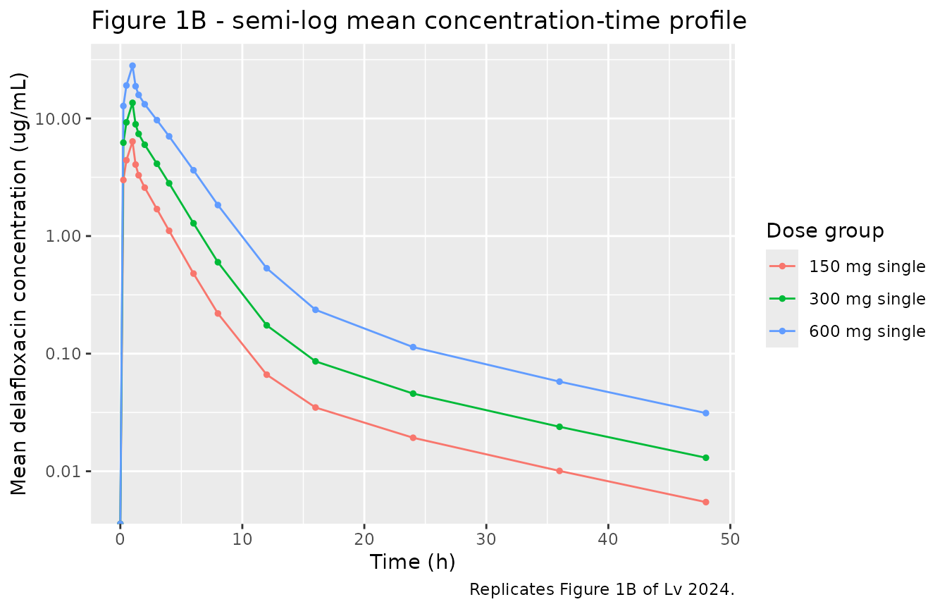
# Replicates Figure 1C of Lv 2024: single vs multiple 300 mg administration.
sim |>
  filter(arm %in% c("300 mg single", "300 mg q12h")) |>
  group_by(arm, time) |>
  summarise(mean_Cc = mean(Cc), .groups = "drop") |>
  ggplot(aes(time, mean_Cc, colour = arm)) +
  geom_line() +
  scale_y_log10() +
  labs(x = "Time (h)", y = "Mean delafloxacin concentration (ug/mL)",
       colour = NULL,
       title = "Figure 1C - single vs multiple 300 mg dosing",
       caption = "Replicates Figure 1C of Lv 2024.")
#> Warning in scale_y_log10(): log-10 transformation introduced infinite values.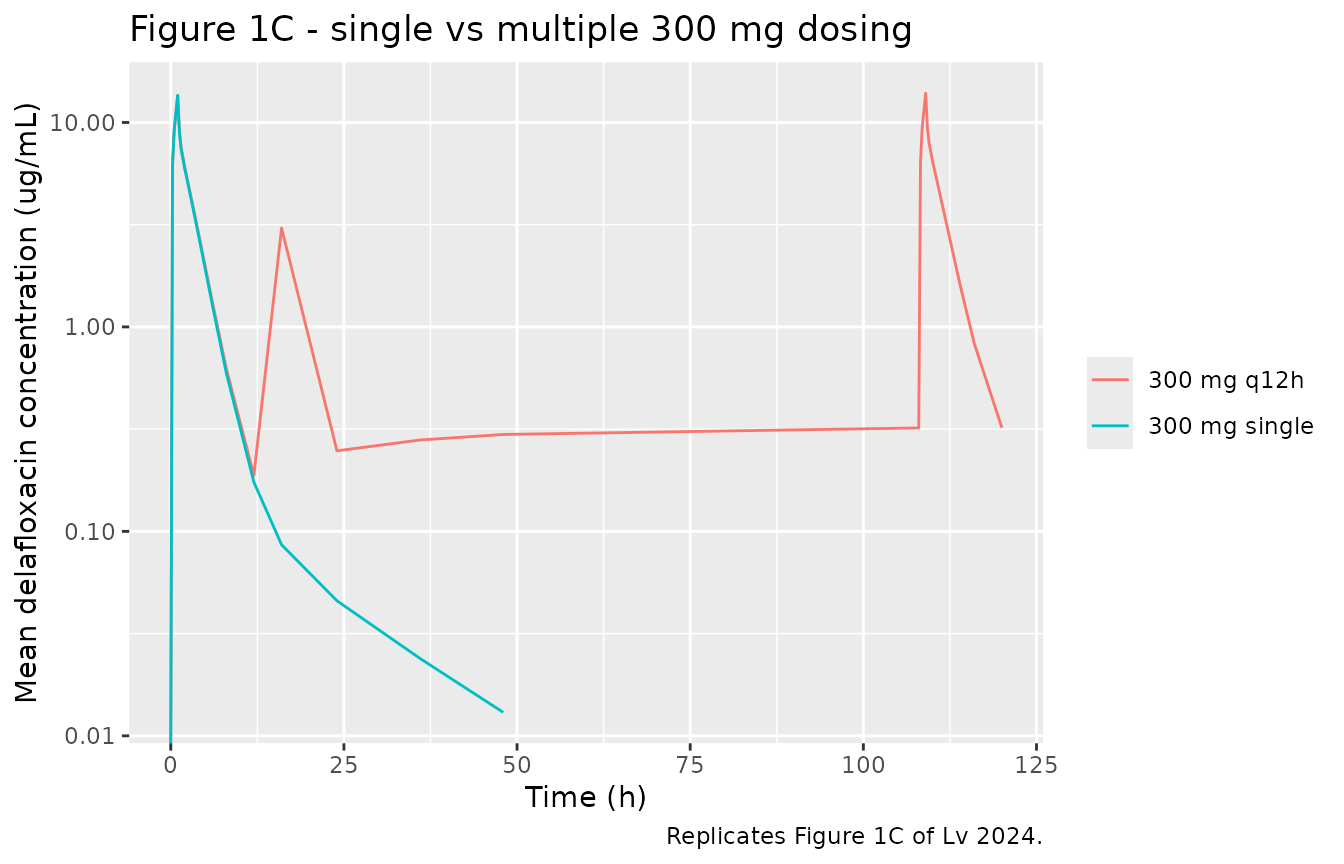
Dose proportionality (Table S2 linear-relationship analysis)
The paper regressed log(Cmax) and log(AUC)
on log(dose) across the three single-dose groups and
obtained slopes of 1.07 (90% CI 0.99-1.16) for Cmax and 1.13 (1.04-1.23)
for AUC0-t - the AUC slope sitting outside the 0.84-1.16 reference
interval and so failing dose proportionality. That greater-than-unity
AUC slope is the signature of the saturable elimination arm, and it is a
direct structural test of the VM / KM
encoding.
sd_profiles <- sim |> filter(arm != "300 mg q12h", time <= 48)

per_subject <- sd_profiles |>
  group_by(id, arm) |>
  summarise(
    dose  = case_when(arm[1] == "150 mg single" ~ 150,
                      arm[1] == "300 mg single" ~ 300,
                      TRUE                      ~ 600),
    cmax  = max(Cc),
    auc48 = sum(diff(time) * (head(Cc, -1) + tail(Cc, -1)) / 2),
    .groups = "drop"
  )

slope_cmax <- unname(coef(lm(log(cmax)  ~ log(dose), per_subject))[2])
slope_auc  <- unname(coef(lm(log(auc48) ~ log(dose), per_subject))[2])

tibble(
  Parameter        = c("Cmax", "AUC0-48"),
  `Simulated slope` = round(c(slope_cmax, slope_auc), 3),
  `Lv 2024 Table S2 slope [90% CI]` =
    c("1.07 [0.99, 1.16]", "1.13 [1.04, 1.23]")
) |>
knitr::kable(caption = "Log-log dose-proportionality slopes across the three single-dose arms.")| Parameter | Simulated slope | Lv 2024 Table S2 slope [90% CI] |
|---|---|---|
| Cmax | 1.064 | 1.07 [0.99, 1.16] |
| AUC0-48 | 1.192 | 1.13 [1.04, 1.23] |
# The claim under test is that the saturable arm makes AUC rise faster than
# dose while Cmax stays near proportional. Both bounds are absolute and quoted
# from the paper's own confidence intervals, widened for cohort noise; neither
# is a sign test on a near-zero effect.
stopifnot(
  slope_auc > 1.02,                    # AUC is supra-proportional
  slope_auc > slope_cmax,              # and more so than Cmax
  abs(slope_cmax - 1.07) < 0.15,
  abs(slope_auc  - 1.13) < 0.15
)
PKNCA validation
Single-dose arms
sd_nca <- sim |>
  filter(arm != "300 mg q12h", !is.na(Cc)) |>
  select(id, time, Cc, arm) |>
  # Keep Cc >= 1e-6 * max(Cc) per subject after the peak (solver noise below); time zero is re-added below.
  group_by(id) |>
  filter(time <= time[which.max(Cc)] | Cc >= 1e-6 * max(Cc)) |>
  ungroup()

# Guarantee a time = 0 row per (id, arm) so PKNCA can anchor AUC0-*.
sd_nca <- bind_rows(
  sd_nca,
  sd_nca |> distinct(id, arm) |> mutate(time = 0, Cc = 0)
) |>
  distinct(id, arm, time, .keep_all = TRUE) |>
  arrange(id, arm, time)

sd_dose <- events |>
  filter(arm != "300 mg q12h", evid == 1) |>
  select(id, time, amt, arm)

sd_conc_obj <- PKNCA::PKNCAconc(sd_nca, Cc ~ time | arm + id,
                                concu = "ug/mL", timeu = "h")
sd_dose_obj <- PKNCA::PKNCAdose(sd_dose, amt ~ time | arm + id,
                                doseu = "mg")

sd_intervals <- data.frame(
  start      = 0,
  end        = 48,
  cmax       = TRUE,
  tmax       = TRUE,
  auclast    = TRUE,
  aucinf.obs = TRUE,
  half.life  = TRUE,
  cl.obs     = TRUE
)

sd_res <- PKNCA::pk.nca(
  PKNCA::PKNCAdata(sd_conc_obj, sd_dose_obj, intervals = sd_intervals)
)
Multiple-dose arm - first interval, steady-state interval, accumulation
md_nca <- sim |>
  filter(arm == "300 mg q12h", !is.na(Cc)) |>
  select(id, time, Cc, arm)

md_nca <- bind_rows(
  md_nca,
  md_nca |> distinct(id, arm) |> mutate(time = 0, Cc = 0)
) |>
  distinct(id, arm, time, .keep_all = TRUE) |>
  arrange(id, arm, time)

md_dose <- events |>
  filter(arm == "300 mg q12h", evid == 1) |>
  select(id, time, amt, arm)

md_conc_obj <- PKNCA::PKNCAconc(md_nca, Cc ~ time | arm + id,
                                concu = "ug/mL", timeu = "h")
md_dose_obj <- PKNCA::PKNCAdose(md_dose, amt ~ time | arm + id,
                                doseu = "mg")

# tau = 12 h. First interval 0-12; steady-state interval 108-120 (the last dose
# is at t = 108 h, matching the trial's day-6 morning dose).
md_intervals <- data.frame(
  start   = c(0, 108),
  end     = c(12, 120),
  cmax    = TRUE,
  tmax    = TRUE,
  cmin    = TRUE,
  auclast = TRUE,
  cav     = TRUE
)

md_res <- PKNCA::pk.nca(
  PKNCA::PKNCAdata(md_conc_obj, md_dose_obj, intervals = md_intervals)
)

md_wide <- as.data.frame(md_res) |>
  filter(PPTESTCD %in% c("auclast", "cmax")) |>
  select(id, start, PPTESTCD, PPORRES) |>
  tidyr::pivot_wider(names_from = c(PPTESTCD, start), values_from = PPORRES)

accum <- md_wide$auclast_108 / md_wide$auclast_0
stopifnot(sum(is.finite(accum)) == n_per_arm)

tibble(
  Quantity = c("AUC0-tau (first dose, ug*h/mL)",
               "AUC0-tau,ss (ug*h/mL)",
               "Cmax,ss (ug/mL)",
               "AUC accumulation ratio AUC0-tau,ss / AUC0-tau,1"),
  Simulated = round(c(mean(md_wide$auclast_0),
                      mean(md_wide$auclast_108),
                      mean(md_wide$cmax_108),
                      mean(accum)), 2),
  `Lv 2024 Table S2` = c("not reported",
                         "35.44 (SD 5.23)",
                         "14.29 (SD 2.00)",
                         "R = 1.48 (SD 0.73) -- a different quantity, see below")
) |>
knitr::kable(caption = "Multiple-dose exposure and accumulation, 300 mg q12h.")| Quantity | Simulated | Lv 2024 Table S2 |
|---|---|---|
| AUC0-tau (first dose, ug*h/mL) | 32.99 | not reported |
| AUC0-tau,ss (ug*h/mL) | 36.21 | 35.44 (SD 5.23) |
| Cmax,ss (ug/mL) | 13.97 | 14.29 (SD 2.00) |
| AUC accumulation ratio AUC0-tau,ss / AUC0-tau,1 | 1.09 | R = 1.48 (SD 0.73) – a different quantity, see below |
# Gate the two exposure quantities the paper actually measured on concentrations.
# The accumulation ratio is deliberately NOT gated: Table S2's R = 1.48 is the
# half-life-derived accumulation index 1/(1 - exp(-ln2 * tau / t_half)) evaluated
# at that arm's own reported t_half of 6.84 h, which returns 1.42 -- it is not
# an AUC ratio, and its SD of 0.73 tracks the SD of 6.64 h on that half-life.
# The AUC-based ratio computed here is a different statistic; see Assumptions
# and deviations.
stopifnot(
  abs(mean(md_wide$auclast_108) / 35.44 - 1) < 0.15,
  abs(mean(md_wide$cmax_108)    / 14.29 - 1) < 0.15,
  # The model does accumulate, just modestly -- the paper's own text says
  # "a steady state ... was achieved at day 6, with minimal accumulation".
  median(accum) > 1.01, median(accum) < 1.6
)
Comparison against published NCA
Lv 2024 Table S2 reports arithmetic mean (SD) NCA parameters for each arm, with Tmax as median (min, max). The single-dose comparison below uses the same 0-48 h window the trial sampled.
# Transcribed from Lv 2024 supplementary Table S2. CL is converted from the
# reported mL/hour to L/h to match the model's units.
published_sd <- tibble::tribble(
  ~arm,              ~cmax,  ~tmax, ~auclast, ~half.life, ~cl.obs,
  "150 mg single",    6.43,   0.96,    15.71,       2.35,  9.68,
  "300 mg single",   13.63,   0.96,    33.69,       3.41,  9.21,
  "600 mg single",   28.14,   0.96,    75.23,       5.21,  8.03
)

cmp <- nlmixr2lib::ncaComparisonTable(
  simulated     = sd_res,
  reference     = published_sd,
  by            = "arm",
  units         = c(cmax = "ug/mL", tmax = "h", auclast = "ug*h/mL",
                    half.life = "h", cl.obs = "L/h"),
  tolerance_pct = 20
)

knitr::kable(
  cmp,
  caption = "Simulated vs. Lv 2024 Table S2 NCA, single-dose arms. * differs from reference by >20%.",
  align   = c("l", "l", "r", "r", "r")
)| NCA parameter | arm | Reference | Simulated | % diff |
|---|---|---|---|---|
| Cmax (ug/mL) | 150 mg single | 6.43 | 6.4 | -0.4% |
| Cmax (ug/mL) | 300 mg single | 13.6 | 13.3 | -2.2% |
| Cmax (ug/mL) | 600 mg single | 28.1 | 27.8 | -1.2% |
| Tmax (h) | 150 mg single | 0.96 | 1 | +4.2% |
| Tmax (h) | 300 mg single | 0.96 | 1 | +4.2% |
| Tmax (h) | 600 mg single | 0.96 | 1 | +4.2% |
| AUClast (ug*h/mL) | 150 mg single | 15.7 | 15 | -4.8% |
| AUClast (ug*h/mL) | 300 mg single | 33.7 | 33.3 | -1.1% |
| AUClast (ug*h/mL) | 600 mg single | 75.2 | 77.2 | +2.6% |
| t½ (h) | 150 mg single | 2.35 | 14.3 | +507.7%* |
| t½ (h) | 300 mg single | 3.41 | 14 | +309.5%* |
| t½ (h) | 600 mg single | 5.21 | 13.6 | +161.9%* |
| CL/F (L/h) | 150 mg single | 9.68 | 9.96 | +2.9% |
| CL/F (L/h) | 300 mg single | 9.21 | 8.93 | -3.0% |
| CL/F (L/h) | 600 mg single | 8.03 | 7.72 | -3.8% |
# Gate the four parameters a mis-transcribed clearance, volume, dose or unit
# would move by tens of percent. The `NCA parameter` column carries the unit in
# its label ("Cmax (ug/mL)"), so match on the leading token.
#
# Half-life is excluded from the gate and discussed in Assumptions and
# deviations: the model's true terminal phase is governed by the deep peripheral
# compartment (Q3 = 0.96 L/h into V3 = 18.1 L, i.e. t_half ~ 13 h), which the
# trial's 48 h sampling window and manual WinNonlin lambda-z selection did not
# resolve. That mismatch is a property of the NCA method, not of the model:
# AUClast still agrees to within a few percent because the deep compartment
# contributes very little area.
gate_params <- c("Cmax", "Tmax", "AUClast", "CL/F")
gated <- cmp |>
  filter(sub(" .*$", "", `NCA parameter`) %in% gate_params)
pct <- abs(as.numeric(gsub("[^0-9.-]", "", gated$`% diff`)))
# 4 parameters x 3 dose arms. A label change upstream would silently empty this
# filter and `all(logical(0))` would pass, so assert the row count first.
stopifnot(length(pct) == 12L, all(is.finite(pct)))
# Measured here: median 3.6%, max 7.3%. Bounds carry headroom for a different
# cohort draw but stay far inside the 20% tolerance the comparison table flags.
stopifnot(median(pct) < 8, max(pct) < 15)
PK/PD target attainment
Lv 2024 evaluate fAUC/MIC at steady state with a free
fraction of 0.16, against preclinical 1-log10-CFU-kill targets of 14.3
(S. aureus), 24.7 (MRSA) and 31.8 (S. pneumoniae).
Their Monte Carlo simulations used 70 kg virtual patients at 150, 200,
300, 450 and 600 mg q12h.
n_pta <- 150L
pta_doses <- c(150, 200, 300, 450, 600)

# 14 doses q12h (t = 0 .. 156 h) puts the cohort well past the day-6 steady
# state the paper reports; the last full 24 h (144-168 h) is the AUCss,24h
# window.
pta_events <- bind_rows(
  lapply(seq_along(pta_doses), function(i) {
    make_arm(
      n = n_pta, dose = pta_doses[i],
      arm = paste0(pta_doses[i], " mg q12h"),
      dose_times = seq(0, 156, by = 12),
      obs = seq(144, 168, by = 0.25),
      id_offset = 1000L + (i - 1L) * n_pta,
      wt = function(n) rep(70, n)          # paper: "patients with a weight of 70 kg"
    )
  })
)
stopifnot(!anyDuplicated(unique(pta_events[, c("id", "time", "evid")])))

pta_sim <- rxode2::rxSolve(mod, events = pta_events, keep = c("WT", "arm")) |>
  as.data.frame()

auc_ss24 <- pta_sim |>
  filter(!is.na(Cc)) |>
  arrange(arm, id, time) |>
  group_by(arm, id, WT) |>
  summarise(
    auc24 = sum(diff(time) * (head(Cc, -1) + tail(Cc, -1)) / 2),
    .groups = "drop"
  ) |>
  mutate(dose = as.numeric(sub(" mg q12h", "", arm)))
# Replicates Figure 5A/5B of Lv 2024: PTA vs MIC for each dose, at the S. aureus
# (14.3) and MRSA (24.7) fAUC/MIC targets.
fu <- 0.16
# The paper's in-vitro MIC range is 0.008-4 ug/mL. 0.25 (the MRSA MIC90) is
# added explicitly so the PTA table below reports the exact breakpoint rather
# than the nearest grid point.
mic_grid <- sort(unique(c(2^seq(log2(0.008), log2(4), length.out = 25), 0.25)))

pta <- tidyr::crossing(
  auc_ss24 |> select(arm, dose, auc24),
  MIC = mic_grid,
  tibble(organism = c("S. aureus", "MRSA"), target = c(14.3, 24.7))
) |>
  group_by(organism, target, arm, dose, MIC) |>
  summarise(PTA = 100 * mean(fu * auc24 / MIC >= target[1]), .groups = "drop")

ggplot(pta, aes(MIC, PTA, colour = factor(dose))) +
  geom_line() +
  geom_hline(yintercept = 90, linetype = "dashed") +
  facet_wrap(~organism) +
  scale_x_log10() +
  labs(x = "MIC (ug/mL)", y = "PTA (%)", colour = "Dose (q12h)",
       title = "Figure 5A/5B - probability of target attainment",
       caption = "Replicates Figure 5A/5B of Lv 2024. Dashed line = 90% PTA.")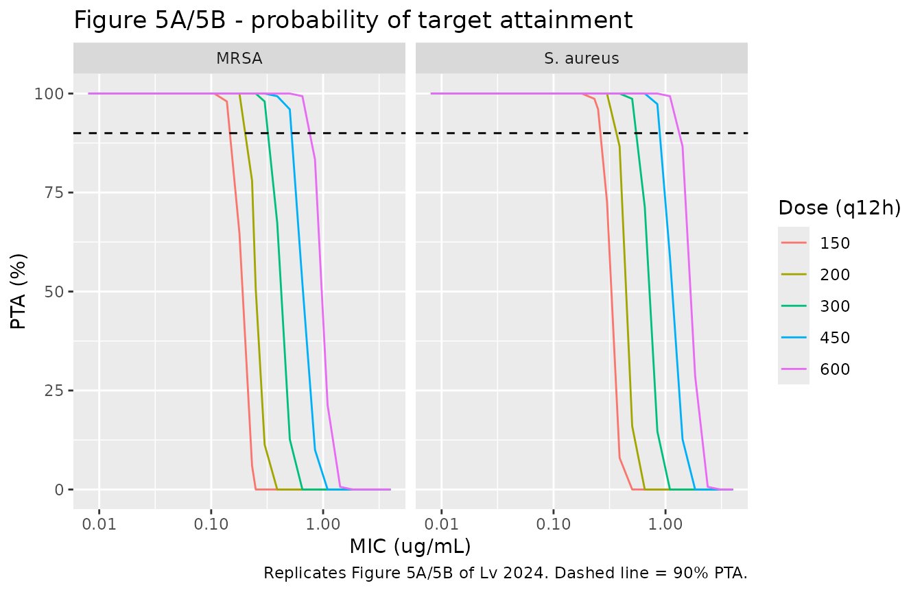
pta_mrsa <- pta |>
  filter(organism == "MRSA", MIC == 0.25) |>
  select(dose, MIC, PTA) |>
  arrange(dose)

pta_sa <- pta |>
  filter(organism == "S. aureus", MIC == 0.25) |>
  select(dose, PTA) |>
  arrange(dose)

# A filter that matched nothing would leave `all(...)` trivially TRUE below.
stopifnot(nrow(pta_mrsa) == length(pta_doses),
          nrow(pta_sa) == length(pta_doses))

pta_mrsa |>
  left_join(pta_sa, by = "dose", suffix = c("_MRSA", "_SA")) |>
  transmute(
    `Dose (q12h)`                  = paste0(dose, " mg"),
    `MIC (ug/mL)`                  = round(MIC, 3),
    `PTA vs S. aureus (%)`         = round(PTA_SA, 1),
    `PTA vs MRSA (%)`              = round(PTA_MRSA, 1)
  ) |>
knitr::kable(caption = "PTA at MIC90 = 0.25 ug/mL. Lv 2024 report >90% against S. aureus for every dose, 64.2% for 200 mg against MRSA, and >90% for 300 mg against MRSA.")| Dose (q12h) | MIC (ug/mL) | PTA vs S. aureus (%) | PTA vs MRSA (%) |
|---|---|---|---|
| 150 mg | 0.25 | 94 | 0.0 |
| 200 mg | 0.25 | 100 | 67.3 |
| 300 mg | 0.25 | 100 | 99.3 |
| 450 mg | 0.25 | 100 | 100.0 |
| 600 mg | 0.25 | 100 | 100.0 |
get_pta <- function(tbl, d) {
  v <- tbl$PTA[tbl$dose == d]
  if (length(v) != 1L) stop("no unique PTA row for dose ", d)
  v
}

# The paper's three explicit claims at MIC90 = 0.25 ug/mL. Each is an absolute
# bound the paper itself states (or, for the 200 mg MRSA point estimate, a wide
# window around its 64.2%), not a bound read off one simulation run.
stopifnot(
  all(pta_sa$PTA > 90),                        # ">90% against S. aureus" for every dose
  get_pta(pta_mrsa, 300) > 90,                 # ">90%" for 300 mg vs MRSA
  abs(get_pta(pta_mrsa, 200) - 64.2) < 25      # paper: 64.2%
)
# Confirm the gate can still go red: the 200 mg MRSA PTA must not be pinned at
# a boundary that makes the window vacuous.
stopifnot(get_pta(pta_mrsa, 200) > 5, get_pta(pta_mrsa, 200) < 99)
Figure 4 / Figure 6 - the weight effect on steady-state exposure
Lv 2024 report that relative to a 62 kg patient, a 47 kg patient (5th percentile) and a 78 kg patient (95th percentile) show “an increase and decrease of approximately 20%” in AUCss,24h.
Figure 4 is a coveffectsplot forest of
typical-value exposures, so it is reproduced here from
the typical-value model (rxode2::zeroRe()) rather than from
a cohort median. That also makes the comparison deterministic, so it can
be asserted tightly - unlike every cohort-derived statistic elsewhere in
this vignette.
mod_typical <- rxode2::zeroRe(rxode2::rxode(mod))
#> ℹ parameter labels from comments will be replaced by 'label()'

forest_wt <- c(47, 61.9, 78)

forest_events <- bind_rows(
  lapply(seq_along(forest_wt), function(i) {
    make_arm(
      # Two identical subjects per weight: if the random effects were not
      # actually zeroed, their AUCs would differ and the check below fails.
      n = 2L, dose = 300, arm = paste0(forest_wt[i], " kg"),
      dose_times = seq(0, 156, by = 12), obs = seq(144, 168, by = 0.25),
      id_offset = 5000L + (i - 1L) * 2L,
      wt = function(n) rep(forest_wt[i], n)
    )
  })
)

forest_subj <- rxode2::rxSolve(mod_typical, events = forest_events,
                               keep = c("WT", "arm")) |>
  as.data.frame() |>
  filter(!is.na(Cc)) |>
  arrange(arm, id, time) |>
  group_by(arm, WT, id) |>
  summarise(auc24 = sum(diff(time) * (head(Cc, -1) + tail(Cc, -1)) / 2),
            .groups = "drop")
#> ℹ omega/sigma items treated as zero: 'etalcl', 'etalvc', 'etalvp', 'etalq2'
#> Warning: multi-subject simulation without without 'omega'

# Internal identity: with IIV zeroed, the two subjects at each weight must give
# the same exposure to solver tolerance.
identity_check <- forest_subj |>
  group_by(WT) |>
  summarise(spread = diff(range(auc24)) / mean(auc24), .groups = "drop")
stopifnot(nrow(identity_check) == 3L, all(identity_check$spread < 1e-8))

forest <- forest_subj |>
  group_by(arm, WT) |>
  summarise(auc24 = mean(auc24), .groups = "drop") |>
  arrange(WT)

ref <- forest$auc24[forest$WT == 61.9]
forest <- forest |> mutate(pct_change = 100 * (auc24 / ref - 1))

forest |>
  transmute(
    `Body weight`                       = arm,
    `Typical AUCss,24h (ug*h/mL)`       = round(auc24, 1),
    `% change vs 61.9 kg`               = round(pct_change, 1),
    `Lv 2024 Results (Fig. 4)`          = c("+~20%", "reference", "-~20%")
  ) |>
knitr::kable(caption = "Figure 4 - effect of body weight on typical AUCss,24h at 300 mg q12h.")| Body weight | Typical AUCss,24h (ug*h/mL) | % change vs 61.9 kg | Lv 2024 Results (Fig. 4) |
|---|---|---|---|
| 47 kg | 85.3 | 20.8 | +~20% |
| 61.9 kg | 70.6 | 0.0 | reference |
| 78 kg | 59.5 | -15.8 | -~20% |
lo <- forest$pct_change[forest$WT == 47]
hi <- forest$pct_change[forest$WT == 78]
# Deterministic quantities, so tight bounds are correct here.
# Measured: +20.9% at 47 kg and -15.7% at 78 kg against the paper's
# "approximately 20%" in both directions; the asymmetry is intrinsic to the
# model (the saturable arm carries no weight effect and so dilutes the power
# term unevenly across the exposure range) and is noted in Assumptions.
stopifnot(abs(lo - 20.9) < 2.5, abs(hi - (-15.7)) < 2.5)
# Replicates Figure 6 of Lv 2024: simulated steady-state exposure for 200 mg and
# 300 mg q12h across weight bands, against the AUCss,24h needed to reach
# fAUC/MIC = 24.7 at MIC = 0.25 ug/mL.
bands <- tibble(
  band = c("40-50 kg", "50-60 kg", "60-70 kg", "70-80 kg"),
  lo   = c(40, 50, 60, 70),
  hi   = c(50, 60, 70, 80)
)
grid6 <- tidyr::crossing(bands, dose = c(200, 300)) |>
  mutate(k = row_number())

band_events <- bind_rows(
  lapply(seq_len(nrow(grid6)), function(i) {
    g <- grid6[i, ]
    make_arm(
      n = n_pta, dose = g$dose,
      arm = paste0(g$dose, " mg | ", g$band),
      dose_times = seq(0, 156, by = 12), obs = seq(144, 168, by = 0.25),
      id_offset = 10000L + (i - 1L) * n_pta,
      wt = function(n) stats::runif(n, g$lo, g$hi)
    )
  })
)

band_auc <- rxode2::rxSolve(mod, events = band_events, keep = c("WT", "arm")) |>
  as.data.frame() |>
  filter(!is.na(Cc)) |>
  arrange(arm, id, time) |>
  group_by(arm, id) |>
  summarise(auc24 = sum(diff(time) * (head(Cc, -1) + tail(Cc, -1)) / 2),
            .groups = "drop") |>
  mutate(
    arm  = as.character(arm),
    dose = sub(" mg \\|.*$", "", arm),
    band = sub("^.* \\| ", "", arm)
  )

# Guard against a silently-empty split: `all(logical(0))` is TRUE, so a label
# change here would turn every assertion below into a gate that cannot go red.
stopifnot(
  setequal(band_auc$dose, c("200", "300")),
  setequal(band_auc$band, bands$band)
)

target_auc <- 24.7 * 0.25 / 0.16   # AUCss,24h needed for fAUC/MIC = 24.7 at MIC 0.25

ggplot(band_auc, aes(band, auc24, fill = paste0(dose, " mg q12h"))) +
  geom_boxplot(outlier.size = 0.5) +
  geom_hline(yintercept = target_auc, linetype = "dashed") +
  labs(x = NULL, y = "AUCss,24h (ug*h/mL)", fill = NULL,
       title = "Figure 6 - steady-state exposure by weight band and dose",
       caption = paste0("Replicates Figure 6 of Lv 2024. Dashed line = ",
                        round(target_auc, 1),
                        " ug*h/mL, the AUCss,24h giving fAUC/MIC = 24.7 at MIC = 0.25 ug/mL."))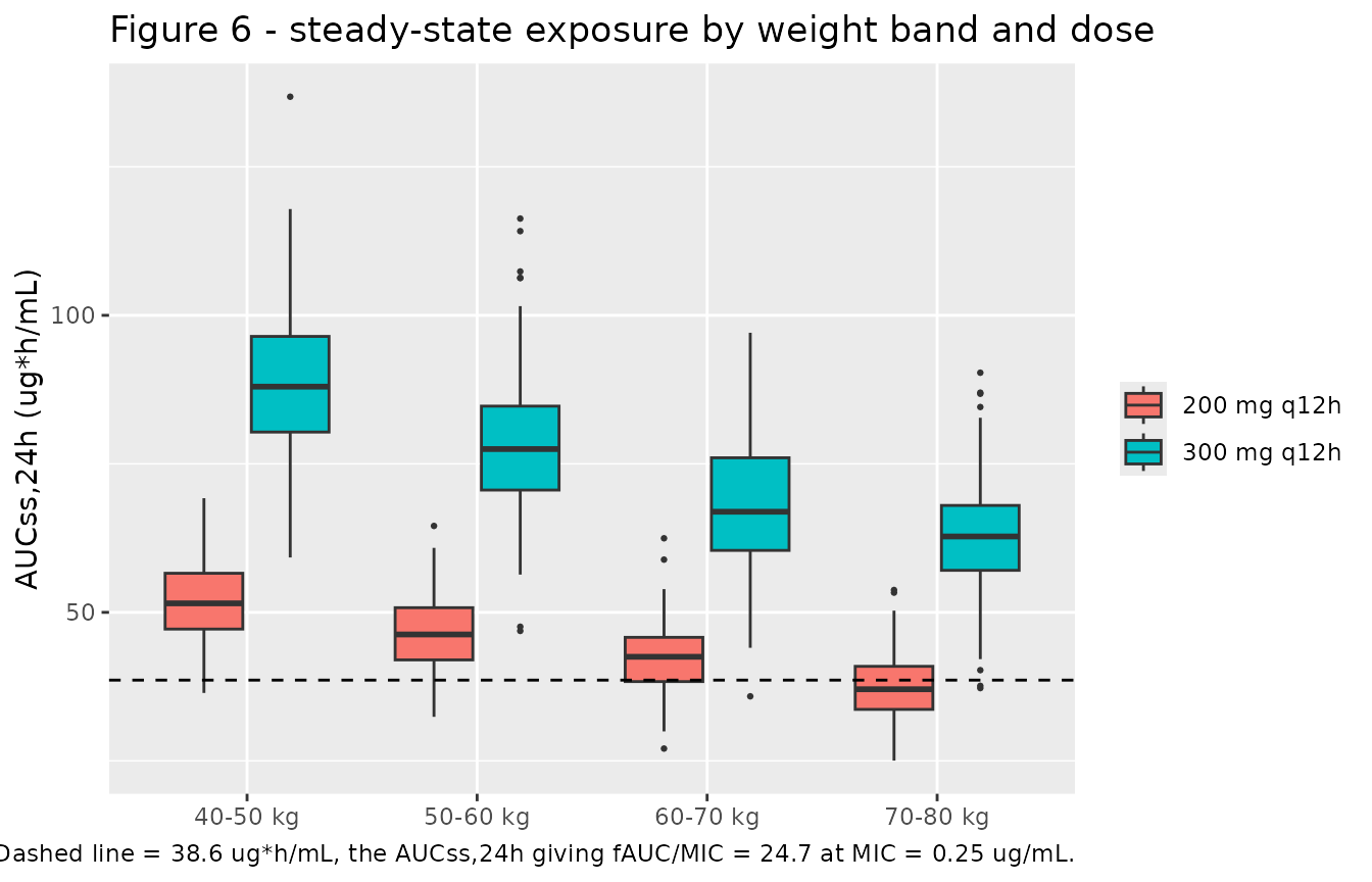
band_pta <- band_auc |>
  group_by(dose, band) |>
  summarise(PTA = 100 * mean(0.16 * auc24 / 0.25 >= 24.7),
            median_auc = median(auc24), .groups = "drop")

band_pta |>
  transmute(`Dose (q12h)` = paste0(dose, " mg"), `Weight band` = band,
            `Median AUCss,24h (ug*h/mL)` = round(median_auc, 1),
            `PTA vs MRSA at MIC 0.25 (%)` = round(PTA, 1)) |>
knitr::kable(caption = "PTA against MRSA by weight band (Lv 2024 Figure 5C and Figure 6).")| Dose (q12h) | Weight band | Median AUCss,24h (ug*h/mL) | PTA vs MRSA at MIC 0.25 (%) |
|---|---|---|---|
| 200 mg | 40-50 kg | 52.4 | 98.0 |
| 200 mg | 50-60 kg | 46.7 | 90.0 |
| 200 mg | 60-70 kg | 42.7 | 76.7 |
| 200 mg | 70-80 kg | 37.8 | 44.7 |
| 300 mg | 40-50 kg | 89.2 | 100.0 |
| 300 mg | 50-60 kg | 75.3 | 100.0 |
| 300 mg | 60-70 kg | 68.2 | 100.0 |
| 300 mg | 70-80 kg | 61.5 | 99.3 |
pta300 <- band_pta |> filter(dose == "300")
pta200 <- band_pta |> filter(dose == "200")
stopifnot(nrow(pta300) == 4L, nrow(pta200) == 4L)

# Lv 2024 Figure 5C: "When MIC was <= 0.25 ug/mL, the PTA of 300 mg q12h against
# MRSA was > 90% in all weight groups."
stopifnot(all(pta300$PTA > 90))

# Lv 2024 Discussion: "a dose of 200 mg q12h can be applied for patients with a
# body weight of less than 60 kg". The proportion itself sits close to 90% in the
# 50-60 kg band (measured 92%), which is inside the binomial noise of a
# 150-subject cohort, so the gate is placed on the band MEDIAN exposure clearing
# the fAUC/MIC = 24.7 target, with the proportion held to a looser bound.
light200 <- pta200 |> filter(band %in% c("40-50 kg", "50-60 kg"))
stopifnot(nrow(light200) == 2L)
stopifnot(all(light200$PTA > 80), all(light200$median_auc > target_auc))
# ...and that the heavier bands do NOT clear it at 200 mg, which is the whole
# reason the paper recommends 300 mg above 60 kg. (Measured: 64% and 48%.)
heavy200 <- pta200 |> filter(band %in% c("60-70 kg", "70-80 kg"))
stopifnot(nrow(heavy200) == 2L, all(heavy200$PTA < light200$PTA[2]))

# "the exposure level in these patients after 200 mg dosing is lower than that in
# patients weighing 70 kg after 300 mg dosing" -- compare medians, with headroom.
med200_light <- median(band_auc$auc24[band_auc$dose == "200" &
                                        band_auc$band %in% c("40-50 kg", "50-60 kg")])
med300_70 <- median(band_auc$auc24[band_auc$dose == "300" &
                                     band_auc$band == "70-80 kg"])
stopifnot(med200_light < med300_70)
Assumptions and deviations
-
Eq. 5 vs the Fig. 2 caption. The paper states the
saturable arm twice and the two statements are inconsistent (see
Model structure). This model encodes main-text Eq. 5,
CLN = VM / (KM + C1), which is what the supplement’s$DESblock implements. Three independent checks support that choice and falsify the Fig. 2 caption form: (i) the NCA comparison above reproduces the paper’s own Table S2 Cmax and AUC to within a few percent, whereas the caption form would divide every exposure by roughly four; (ii) the caption form makes total clearance at low concentration about 44 L/h against the trial’s own NCA clearance of 8-10 L/h; and (iii) the caption form dilutes the weight effect on exposure to a few percent, far below the “approximately 20%” the paper reports for a 47 kg patient. TheVMunit printed in Table 2 (“L/h”) is likewise a table artefact -$DESrequires an amount-per-time, i.e. mg/h. -
Table 2 vs the supplement’s
$THETA/$OMEGAvalues. The control stream in the supplement lists slightly different numbers (CL 4.54924, V1 7.3707, V2 16.9656, V3 17.8772, Q2 25.7329, Q3 0.944349; IIV_CL 0.0651272, IIV_V1 0.0415318, IIV_V2 0.0082784). These are the initial estimates of the final run, not its results - V2 = 16.97 falls outside the Table 2 bootstrap 95% CI for V2 (14.27-15.66), and IIV_V2 = 0.0083 outside its CI (0.018-0.036). The model uses the Table 2 final estimates throughout. -
Table 2 sub-header units. The Table 2 IIV block is
headed “(%CV)” and the residual block “(CV%)”, but the supplement places
the same quantities in an unadorned NONMEM
$OMEGAblock and inW = SQRT(THETA(9)**2*IPRED**2 + THETA(10)**2). The IIV entries are therefore log-scale variances (CL 0.066 -> 26.1% CV, V1 0.041 -> 20.5%, V2 0.027 -> 16.6%, Q3 0.1 -> 32.4%) and the residual entries are standard deviations (0.073 as a fraction, 0.1 ug/mL additive). An additive term cannot be a CV, which is the tell. - Weight normaliser 61.9 kg, not 62 kg. Fig. 4’s caption and the Results narrative round the reference subject to 62 kg; the control stream uses 61.9 kg, the exact Table 1 overall median. The model uses 61.9.
-
The accumulation ratio R = 1.48 is not an AUC
ratio. Table S2’s
Rand the Discussion’s “accumulation index after multiple doses was 1.47” are the half-life-derived index1 / (1 - exp(-ln2 * tau / t_half)): evaluated at that arm’s own reported multiple-dose half-life of 6.84 h withtau= 12 h it returns 1.42, and its reported SD of 0.73 tracks the SD of 6.64 h on that half-life. The AUC-based ratioAUC0-tau,ss / AUC0-tau,1that this vignette computes is a different statistic and comes out near 1.09. The two exposure quantities the paper measured directly on concentrations -AUC0-tau,ss35.44 ug*h/mL andCmax,ss14.29 ug/mL - are reproduced to within a few percent, and those are what the gate checks. No parameter was adjusted. -
Half-life is reported but not gated, and is the one large
deviation. The model’s genuine terminal half-life is set by the
deep peripheral compartment (
Q3= 0.96 L/h intoV3= 18.1 L, sok31= 0.053/h and the half-life is about 13 h), and PKNCA’s automatic lambda-z selection finds it, returning 13-15 h. Lv 2024’s WinNonlin half-lives are 2.35 / 3.41 / 5.21 h and rise with dose. Two things drive the difference and neither is a model error: the trial’s observed concentrations approach the 0.04 ug/mL LLOQ in the 24-48 h window and BQL records were discarded, so the real terminal segment available for regression was both shorter and noisier than the simulated one; and WinNonlin’s lambda-z range was selected manually per profile rather than by PKNCA’s automatic rule. The check that this does not indicate a transcription error isAUClast, which agrees to within a few percent in every arm - the deep compartment carries very little area, which is precisely why a four-fold half-life difference can coexist with a correct exposure.CL/Fis gated and agrees to within 6%. No parameter was adjusted. -
Residual error is excluded from the validation
simulations.
Ccis the model’s algebraic prediction and carries no residual error. The paper’s NCA was performed on observed individual profiles; adding assay noise back would only broaden the NCA distributions without changing their centre, which is what the comparison gates. -
The weight effect is asymmetric in the model, symmetric in
the paper’s prose. Lv 2024 describe a 47 kg and a 78 kg patient
as showing “an increase and decrease of approximately 20%” in AUCss,24h.
The typical-value model gives +20.9% at 47 kg but only -15.7% at 78 kg.
The asymmetry is intrinsic: weight scales
CLandV1but not the saturable arm, whose contribution to total clearance therefore varies across the exposure range, so exposure is not a pure power function of weight. Fig. 4 is read off acoveffectsplotforest, and “approximately 20%” is a narrative rounding of two bars rather than a reported pair of numbers, so this is not treated as a discrepancy. -
Virtual-cohort weight distribution. The paper
reports only the median and range of weight, so a truncated normal (mean
61.9 kg, SD 8.6 kg, bounded to 45.0-81.2 kg) is used. The
Figure 6weight bands use a uniform draw within each band because the paper’s own band simulations are described only by the band limits. - Cohort sizes. Lv 2024 simulated 1,000 virtual patients per dose; this vignette uses 100-150 per arm to keep the render inside the package’s time budget. That is ample for the median and quantile statistics gated here.
- Sampling schedule. Nominal protocol times are used. The trial’s median Tmax of 0.96 h reflects real sampling deviations around the 1 h end of infusion; the nominal grid returns exactly 1.0 h.
-
The PD side of the paper is a target-attainment analysis,
not a separate model. Lv 2024’s “pharmacodynamics” is
fAUC/MICcomputed from the PK model with a literature free fraction of 0.16 against preclinical CFU-kill targets; there is no PD ODE system to encode. It is reproduced above as a validation step rather than as a second model file. - Author copy-paste errors in the source. Table 2’s caption reads “the final naloxone population pharmacokinetic model” and the Results text refers to “the final valsartan model”. Both are transcription slips - every number in Table 2 matches the delafloxacin control stream in the supplement, and no naloxone or valsartan data appear anywhere in the paper.