Veliparib (Stodtmann 2021)
Source:vignettes/articles/Stodtmann_2021_veliparib.Rmd
Stodtmann_2021_veliparib.RmdModel and source
- Citation: Stodtmann S., Nuthalapati S., Eckert D., Kasichayanula S., Joshi R., Bach B. A., Mensing S., Menon R., Xiong H. (2021). A Population Pharmacokinetic Meta-Analysis of Veliparib, a PARP Inhibitor, Across Phase 1/2/3 Trials in Cancer Patients. The Journal of Clinical Pharmacology 61(9):1195-1205. doi:10.1002/jcph.1875.
- Description: One-compartment population PK model for the oral PARP inhibitor veliparib (ABT-888) in adults with ovarian cancer, breast cancer or other solid tumours, pooled from 9 phase 1/2/3 studies (meta-analysis of individual-level data, n = 1470). First-order absorption without lag, with multiplicative fed and fasting effects on ka relative to an unknown-prandial-state reference; linear apparent clearance CL/F scaled by Cockcroft-Gault creatinine clearance (capped at 120 mL/min), serum albumin, male sex and strong CYP2D6 inhibitor co-medication; apparent volume Vc/F scaled by body weight, serum albumin and male sex. Separate combined additive-plus-proportional residual errors for the absorption phase (time after dose up to 2.5 h) and the elimination phase.
- Article: https://doi.org/10.1002/jcph.1875 (open access, PMC8453554)
Stodtmann et al. pooled individual veliparib concentrations from nine
AbbVie studies (six phase 1, one phase 2 and two phase 3) into one
population PK analysis. The final model is one-compartment with
first-order absorption and linear clearance. The time base is
days and concentrations are in ug/mL,
exactly as the paper reports them (Table 4: CL/F (L/day),
ka (1/day); additive errors in ug/mL).
The library also contains Niu_2017_veliparib, an earlier
single-study parent-plus-M8 model from a different group (hours, ng/mL,
two compartments). The two models are independent fits to different
data.
Population
The model was fit to 9160 plasma concentrations from 1470 adults (Stodtmann 2021 Table 3, All Subjects): median age 55 years (22-86), median body weight 66.0 kg (35.7-182), 97% female, 75% White, 12% Asian, 4% Black. The subjects had ovarian, fallopian tube or primary peritoneal cancer (58%), breast cancer (38%) or other solid tumours (5%), and received oral veliparib 10-400 mg twice daily, alone or with temozolomide, carboplatin/gemcitabine or carboplatin/paclitaxel (Table 1). Median Cockcroft-Gault creatinine clearance was 96.5 mL/min (28.2-289); 32% had mild and 9% moderate renal impairment. Median serum albumin was 40 g/L (20-52).
The same information is available programmatically via
readModelDb("Stodtmann_2021_veliparib")()$population.
Source trace
Every ini() value carries an in-file comment naming its
row in Table 4. The typical-value equations are printed in the Results
section Significant Covariates:
-
CL/F = 479 * (min(CrCL,120)/120)^0.513 * (ALB/40)^0.427 * 1.20^Male * 0.885^CYP2D6L/day -
Vc/F = 152 * (WTKG/70)^0.505 * (ALB/40)^0.260 * 1.25^MaleL -
ka = 59.4 * 1.11^Fasting * 0.356^Fed1/day
| Parameter | Value | Source location |
|---|---|---|
lka |
log(59.4) 1/day | Table 4 ‘ka (1/day)’ |
lcl |
log(479) L/day | Table 4 ‘CL/F (L/day)’ |
lvc |
log(152) L | Table 4 ‘Vc/F (L)’ |
e_fed_ka |
0.356 | Table 4 ‘Fed on ka’ |
e_fast_ka |
1.11 | Table 4 ‘Fasting on ka’ |
e_crcl_cl |
0.513 | Table 4 ‘Creatinine clearance on CL/F’; cap and reference 120 mL/min from the CL/F equation and Table 2 |
e_alb_cl |
0.427 | Table 4 ‘Albumin on CL/F’; reference 40 g/L from the CL/F equation |
e_male_cl |
1.20 | Table 4 ‘Male on CL/F’ |
e_cyp2d6inh_cl |
0.885 | Table 4 ‘Strong inhibitors of CYP2D6 on CL/F’ |
e_wt_vc |
0.505 | Table 4 ‘Body weight on Vc/F’; reference 70 kg from Table 2 and the Vc/F equation |
e_alb_vc |
0.260 | Table 4 ‘Albumin on Vc/F’ |
e_male_vc |
1.25 | Table 4 ‘Male on Vc/F’ |
etalcl |
0.085 (variance) | Table 4 ‘BSV on CL/F’ (29.8% CV) |
etalvc |
0.064 (variance) | Table 4 ‘BSV on Vc/F’ (25.7% CV) |
addSd_abs, propSd_abs
|
0.004 ug/mL, 0.208 | Table 4 absorption-phase error rows |
addSd_elim, propSd_elim
|
2.96e-7 ug/mL, 0.078 | Table 4 elimination-phase error rows |
| Phase switch at 2.5 h after dose | 2.5/24 day | Results: ‘absorption phase (before Tmax at 2.5 hours)’ |
d/dt(depot), d/dt(central)
|
n/a | Results: ‘1-compartment model with linear clearance and first-order absorption’ |
Covariate effects on steady-state exposure
The paper reports its covariate effects as the change in steady-state
AUC, computed as dose divided by clearance, relative to a reference
subject (female, no strong CYP2D6 inhibitor, CrCL >= 120 mL/min,
albumin 40 g/L; Results and Figure 3). Because
AUCss = Dose / (CL/F), each effect is a pure function of
the typical-value clearance, so the packaged model must reproduce the
printed numbers from its own parameters. The check below reads the
typical CL/F from a typical-value solve of the packaged model (not from
a re-typed formula).
The paper’s values are medians of its bootstrap distribution; the model uses the point estimates. The two agree to within a few tenths of a percentage point for every row, so the gate is 0.5 percentage points.
mod <- readModelDb("Stodtmann_2021_veliparib")
mod_typ <- rxode2::zeroRe(mod)
#> ℹ parameter labels from comments will be replaced by 'label()'
#> Warning: No sigma parameters in the model

scenarios <- tibble::tribble(
  ~scenario, ~CRCL, ~ALB, ~SEXF, ~CONMED_CYP2D6_INH, ~published_pct,
  "Reference", 120, 40, 1, 0, 0,
  "Mild renal impairment (CrCL 75 mL/min)", 75, 40, 1, 0, 27.3,
  "Moderate renal impairment (CrCL 45 mL/min)", 45, 40, 1, 0, 65.4,
  "Male", 120, 40, 0, 0, -16.5,
  "Strong CYP2D6 inhibitor", 120, 40, 1, 1, 13.0,
  "Albumin 45 g/L", 120, 45, 1, 0, -4.91,
  "Albumin 35 g/L", 120, 35, 1, 0, 5.87
) |>
  mutate(id = seq_len(n()), WT = 70, FED = 0, FED_MISSING = 1)

ev_typ <- scenarios |>
  select(id, CRCL, ALB, SEXF, CONMED_CYP2D6_INH, WT, FED, FED_MISSING) |>
  tidyr::crossing(time = c(0, 1)) |>
  mutate(evid = 0L, amt = 0, cmt = "central")

sim_typ <- rxode2::rxSolve(mod_typ, events = ev_typ, keep = "id") |>
  as.data.frame()
#> Warning: 'keep' contains id
#> which are output when needed, ignoring these items
#> ℹ omega/sigma items treated as zero: 'etalcl', 'etalvc'
#> Warning: multi-subject simulation without without 'omega'
cl_typ <- sim_typ |>
  group_by(id) |>
  summarise(cl = first(cl), vc = first(vc), .groups = "drop")

cov_tab <- scenarios |>
  left_join(cl_typ, by = "id") |>
  mutate(
    model_pct = 100 * (cl[scenario == "Reference"] / cl - 1),
    diff_pts = model_pct - published_pct
  )

cov_tab |>
  select(scenario, cl, published_pct, model_pct, diff_pts) |>
  dplyr::rename(
    "Scenario" = scenario,
    "Typical CL/F (L/day)" = cl,
    "Published AUCss change (%)" = published_pct,
    "Model AUCss change (%)" = model_pct,
    "Difference (points)" = diff_pts
  ) |>
knitr::kable(digits = 2, caption = "Replicates the covariate effects of Stodtmann 2021 Results and Figure 3.")| Scenario | Typical CL/F (L/day) | Published AUCss change (%) | Model AUCss change (%) | Difference (points) |
|---|---|---|---|---|
| Reference | 479.00 | 0.00 | 0.00 | 0.00 |
| Mild renal impairment (CrCL 75 mL/min) | 376.38 | 27.30 | 27.27 | -0.03 |
| Moderate renal impairment (CrCL 45 mL/min) | 289.61 | 65.40 | 65.39 | -0.01 |
| Male | 574.80 | -16.50 | -16.67 | -0.17 |
| Strong CYP2D6 inhibitor | 423.91 | 13.00 | 12.99 | -0.01 |
| Albumin 45 g/L | 503.71 | -4.91 | -4.90 | 0.01 |
| Albumin 35 g/L | 452.45 | 5.87 | 5.87 | 0.00 |
stopifnot(
  nrow(cov_tab) == 7L,
  abs(cov_tab$cl[cov_tab$scenario == "Reference"] - 479) < 1e-6,
  all(abs(cov_tab$diff_pts) < 0.5)
)
The Discussion also states that a 10 kg change in body weight changes
Vc/F by only about 7%. Around the 66 kg median,
(76/66)^0.505 = 1.074:
ev_wt <- tibble(id = 1:2, WT = c(66, 76)) |>
  mutate(CRCL = 120, ALB = 40, SEXF = 1, CONMED_CYP2D6_INH = 0, FED = 0, FED_MISSING = 1) |>
  tidyr::crossing(time = c(0, 1)) |>
  mutate(evid = 0L, amt = 0, cmt = "central")
vc_wt <- rxode2::rxSolve(mod_typ, events = ev_wt, keep = "id") |>
  as.data.frame() |>
  group_by(id) |>
  summarise(vc = first(vc), .groups = "drop")
#> Warning: 'keep' contains id
#> which are output when needed, ignoring these items
#> ℹ omega/sigma items treated as zero: 'etalcl', 'etalvc'
#> Warning: multi-subject simulation without without 'omega'
vc_change_pct <- 100 * (vc_wt$vc[2] / vc_wt$vc[1] - 1)
vc_change_pct
#> [1] 7.384395
stopifnot(abs(vc_change_pct - 7) < 1)
Virtual cohort
The observed data are not public. The virtual cohort draws covariates
independently from distributions matched to the Table 3 summaries (All
Subjects), redrawing any value outside the observed range rather than
clamping it. The prandial state is left unknown
(FED_MISSING = 1), as it was for 95% of the fitted
subjects. Three twice-daily regimens used in the phase 2/3 studies are
simulated, 150 subjects each.
set.seed(20210901)
rxode2::rxSetSeed(20210901)

# Draw from a sampler, redrawing values outside [lo, hi].
draw_in_range <- function(n, sampler, lo, hi) {
  x <- sampler(n)
  bad <- x < lo | x > hi
  while (any(bad)) {
    x[bad] <- sampler(sum(bad))
    bad <- x < lo | x > hi
  }
  x
}

make_cohort <- function(n, dose_mg, id_offset) {
  tibble(
    id = id_offset + seq_len(n),
    regimen = paste0(dose_mg, " mg BID"),
    dose = dose_mg,
    WT = draw_in_range(n, function(k) rlnorm(k, log(66), 0.25), 35.7, 182),
    ALB = draw_in_range(n, function(k) rnorm(k, 39.6, 5.05), 20, 52),
    CRCL = draw_in_range(n, function(k) rlnorm(k, log(96.5), 0.34), 28.2, 289),
    SEXF = rbinom(n, 1, 0.97),
    CONMED_CYP2D6_INH = rbinom(n, 1, 0.05),
    FED = 0,
    FED_MISSING = 1
  )
}

n_per_arm <- 150L
cohort <- bind_rows(
  make_cohort(n_per_arm, 120, 0L),
  make_cohort(n_per_arm, 150, n_per_arm),
  make_cohort(n_per_arm, 300, 2L * n_per_arm)
)

# Twice-daily dosing for 7 days (tau = 0.5 day); steady state is reached well
# before the last interval (typical half-life log(2) * 152 / 479 = 0.22 day).
tau <- 0.5
n_dose <- 14L
t_last <- tau * (n_dose - 1)
obs_times <- sort(unique(c(
  seq(0, t_last, by = 0.25),
  t_last + c(0, 0.5, 1, 1.5, 2, 2.5, 3, 4, 5, 6, 8, 10, 12) / 24
)))

doses <- cohort |>
  tidyr::crossing(time = tau * (seq_len(n_dose) - 1)) |>
  mutate(evid = 1L, amt = dose, cmt = "depot")
obs <- cohort |>
  tidyr::crossing(time = obs_times) |>
  mutate(evid = 0L, amt = 0, cmt = "central")
events <- bind_rows(doses, obs) |>
  arrange(id, time, desc(evid)) |>
  select(id, time, evid, amt, cmt, regimen, dose, WT, ALB, CRCL, SEXF,
         CONMED_CYP2D6_INH, FED, FED_MISSING)
stopifnot(!anyDuplicated(events[, c("id", "time", "evid")]))
Simulation
sim <- rxode2::rxSolve(mod, events = events, keep = c("regimen", "dose")) |>
  as.data.frame()
#> ℹ parameter labels from comments will be replaced by 'label()'
stopifnot(!anyNA(sim$Cc))
Steady-state profile
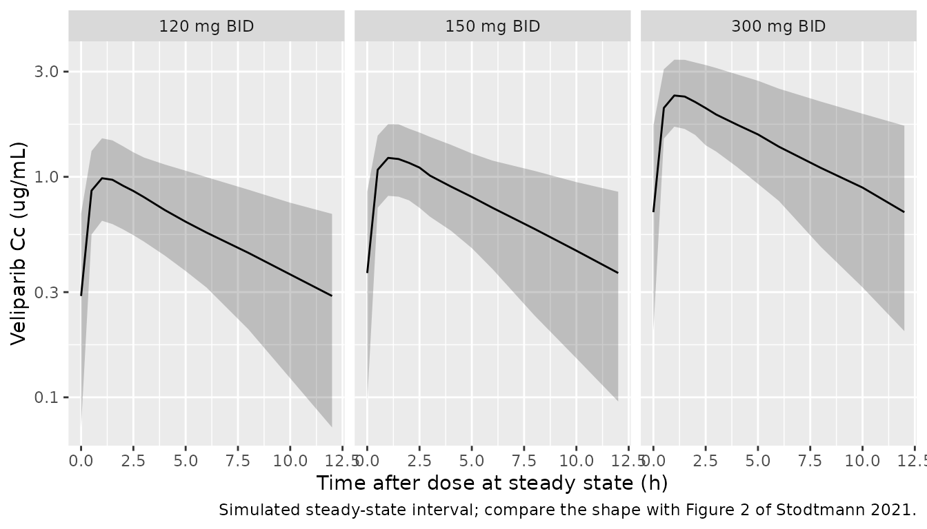
The paper’s Figure 2 is a prediction-corrected VPC over all nine studies, whose dose, food and sampling mix cannot be reconstructed, so it is not overlaid numerically. The plot below shows the simulated steady-state dosing interval of each regimen (individual predictions, 5th/50th/95th percentiles).
sim |>
  filter(time >= t_last) |>
  mutate(tad_h = (time - t_last) * 24) |>
  group_by(regimen, tad_h) |>
  summarise(
    Q05 = quantile(Cc, 0.05), Q50 = median(Cc), Q95 = quantile(Cc, 0.95),
    .groups = "drop"
  ) |>
  ggplot(aes(tad_h, Q50)) +
  geom_ribbon(aes(ymin = Q05, ymax = Q95), alpha = 0.25) +
  geom_line() +
  facet_wrap(~regimen) +
  scale_y_log10() +
  labs(
    x = "Time after dose at steady state (h)", y = "Veliparib Cc (ug/mL)",
    caption = "Simulated steady-state interval; compare the shape with Figure 2 of Stodtmann 2021."
  )
PKNCA validation
Non-compartmental analysis of the last (steady-state) dosing interval, grouped by regimen.
sim_nca <- sim |>
  filter(!is.na(Cc)) |>
  mutate(Cc = pmax(Cc, 0)) |>
  select(id, time, Cc, regimen)

dose_nca <- events |>
  filter(evid == 1, time == t_last) |>
  select(id, time, amt, regimen)

conc_obj <- PKNCA::PKNCAconc(sim_nca, Cc ~ time | regimen + id)
dose_obj <- PKNCA::PKNCAdose(dose_nca, amt ~ time | regimen + id)
intervals <- data.frame(
  start = t_last, end = t_last + tau,
  cmax = TRUE, tmax = TRUE, cmin = TRUE, auclast = TRUE, cav = TRUE
)
nca_res <- PKNCA::pk.nca(PKNCA::PKNCAdata(conc_obj, dose_obj, intervals = intervals))
nca_tab <- as.data.frame(nca_res$result)

nca_tab |>
  group_by(regimen, PPTESTCD) |>
  summarise(median = median(PPORRES), .groups = "drop") |>
  tidyr::pivot_wider(names_from = PPTESTCD, values_from = median) |>
  dplyr::rename(
    "Regimen" = regimen,
    "AUCtau (ug*day/mL)" = auclast,
    "Cavg (ug/mL)" = cav,
    "Cmax (ug/mL)" = cmax,
    "Cmin (ug/mL)" = cmin,
    "Tmax (day)" = tmax
  ) |>
knitr::kable(digits = 3, caption = "Median simulated steady-state NCA by regimen.")| Regimen | AUCtau (ug*day/mL) | Cavg (ug/mL) | Cmax (ug/mL) | Cmin (ug/mL) | Tmax (day) |
|---|---|---|---|---|---|
| 120 mg BID | 0.286 | 0.572 | 0.986 | 0.288 | 0.042 |
| 150 mg BID | 0.372 | 0.744 | 1.220 | 0.366 | 0.042 |
| 300 mg BID | 0.718 | 1.435 | 2.341 | 0.691 | 0.042 |
The paper reports no NCA table. Its exposure metric is
AUCss = Dose / (CL/F), so the simulated per-subject
steady-state AUC over one interval must equal the dose divided by that
subject’s own clearance. This is a mass-balance identity on the solved
ODE; the tolerance covers only the trapezoidal error of the sampling
grid around the absorption peak.
auc_check <- nca_tab |>
  filter(PPTESTCD == "auclast") |>
  left_join(
    sim |> group_by(id) |> summarise(cl = first(cl), dose = first(dose), .groups = "drop"),
    by = "id"
  ) |>
  mutate(pct_diff = 100 * (PPORRES / (dose / cl) - 1))

summary(auc_check$pct_diff)
#>    Min. 1st Qu.  Median    Mean 3rd Qu.    Max.
#> -2.2410 -0.8066 -0.5811 -0.6571 -0.4314 -0.2777
stopifnot(
  nrow(auc_check) == 3L * n_per_arm,
  abs(median(auc_check$pct_diff)) < 3,
  quantile(abs(auc_check$pct_diff), 0.9) < 5
)
Phase-specific residual error
The residual error switches from the absorption-phase terms to the
elimination-phase terms 2.5 h after each dose. Each simulated
observation is standardised by the combined SD that Table 4 implies for
its phase, sqrt(add^2 + (prop * Cc)^2). If the model
applies the right pair of terms in each phase, the standardised
residuals have SD 1 in both phases. Applying the absorption terms late
(or the elimination terms early) moves the SD by a factor of about
2.7.
res <- sim |>
  mutate(
    tad_h = 24 * (time - tau * pmin(floor(time / tau + 1e-9), n_dose - 1)),
    phase = ifelse(tad_h <= 2.5, "absorption (<= 2.5 h)", "elimination (> 2.5 h)"),
    sd_expected = ifelse(
      tad_h <= 2.5,
      sqrt(0.004^2 + (0.208 * Cc)^2),
      sqrt(2.96e-7^2 + (0.078 * Cc)^2)
    ),
    z = (sim - Cc) / sd_expected
  ) |>
  group_by(phase) |>
  summarise(n = n(), sd_z = sd(z), .groups = "drop")
knitr::kable(res, digits = 3, caption = "SD of standardised residuals by phase (expected 1).")| phase | n | sd_z |
|---|---|---|
| absorption (<= 2.5 h) | 8100 | 1.001 |
| elimination (> 2.5 h) | 9450 | 0.996 |
Assumptions and deviations
-
Categorical covariates are multiplicative factors
(
theta^I). The Methods give a generic categorical equationTVP = theta * (1 + I * theta_cat), but the final equations print1.20^Male,0.885^CYP2D6,1.25^Male,1.11^Fastingand0.356^Fed, and the Results’ effect sizes (males -16.5%, strong CYP2D6 inhibitors +13.0% AUCss) are reproduced only by the power form. Under the(1 + theta)form males would have 55% lower AUCss, and food would speed absorption rather than delay it as the Discussion describes. The model follows the printed final equations. -
Residual-error rows are read as standard
deviations. Table 4 does not say whether its RUV estimates are
SDs or variances. The additive rows carry concentration units (ug/mL),
not squared units, and the elimination-phase proportional RSE of 1.44%
is below
sqrt(2/9160) = 1.48%, the smallest RSE a variance estimated from 9160 observations can have. The bootstrap CIs of the RUV rows are wider than their %RSE implies, so the RSEs are not a strong argument by themselves. -
Combined error form. The paper says only “combined
(additive and proportional)”; the nlmixr2 default
(
combined2, variances added) is used. - Absorption-phase boundary. The Results place the switch “before Tmax at 2.5 hours”, and the outlier rule applies to “time since last dose of more than 2.5 hours”, so an observation exactly 2.5 h after the dose is assigned to the absorption phase.
-
Food effect reference level. The published ka (59.4
1/day) is for an unknown prandial state, which covers 95% of the
subjects. It is encoded with
FED_MISSING = 1; setFED_MISSING = 0andFED = 0/1to simulate a defined fasting or fed dose. - Creatinine clearance is raw Cockcroft-Gault in mL/min, not BSA-normalised, and is capped at 120 mL/min inside the model.
- Discussion vs Results. The Discussion quotes a 25% AUCss increase for mild renal impairment where the Results (and the model) give 27.3%. The Figure 3 legend calls CrCL 75 and 45 mL/min “moderate” and “severe”, where the Results call them mild and moderate. Neither affects the model.
- Virtual cohort. Covariates are drawn independently; correlations between body weight, albumin, creatinine clearance and sex were not reported. Sex and strong-CYP2D6-inhibitor frequencies follow Table 3 (3% male, 5% with a strong CYP2D6 inhibitor).
- No erratum or correction notice for this article was found on Europe PMC as of 2026-09-29.