Treprostinil: intravenous PK (Wu 2022)

Model and source

mod <- readModelDb("Wu_2022_treprostinil")
ui <- rxode2::rxode(mod)

• Citation: Wu X, Zhang X, Xu R, Shaik IH, Venkataramanan R. (2022). Physiologically based pharmacokinetic modelling of treprostinil after intravenous injection and extended-release oral tablet administration in healthy volunteers: An extrapolation to other patient populations including patients with hepatic impairment. Br J Clin Pharmacol 88(2):587-599. doi:10.1111/bcp.14966.
• Article: https://doi.org/10.1111/bcp.14966
• Supplement (Supplemental Table 1): https://www.ncbi.nlm.nih.gov/pmc/articles/PMC9290939/

What this model is, and what it is not

Wu 2022 builds a Simcyp (version 17 release 1) physiologically based pharmacokinetic (PBPK) model of the prostacyclin analogue treprostinil. The model has an intravenous arm, built on one infusion study and verified on two more, and an arm for the extended-release oral tablet (Orenitram). The oral arm is then extrapolated to Child-Pugh A/B/C hepatic impairment and to patients with pulmonary arterial hypertension or systemic sclerosis.

Simcyp’s whole-body mass-balance equations are proprietary and appear nowhere in the paper. Distribution uses the full-PBPK layout with Rodgers and Rowland tissue:plasma partition coefficients. Table 3 prints all twelve tissue Kp values, the optimized Kp scalar (0.7) and the optimized adipose Kp (1.20). It prints no organ volume and no blood flow, so the multi-tissue structure cannot be rebuilt. The paper does report, completely, what the intravenous disposition needs:

• the total in vivo intravenous clearance, 43 L/h. This is “the average clearance value after intravenous administration obtained from 3 reports”, and the retrograde clearance model was built to reproduce it (section 2.2);
• its renal component, 0.9 L/h (Table 4);
• the final model’s predicted steady-state volume of distribution, 0.42 L/kg (Table 3);
• and, in Supplemental Table 1, the PBPK model’s own predicted Cmax and AUC for every simulated regimen. These are the answer key for any reduction.

That is enough for a one-compartment intravenous reduction with no fitted parameter. Below, it reproduces the platform’s predicted Cmax and AUC for all three intravenous studies to within 14%.

Why only the intravenous arm

The oral arm cannot be reduced. The reason is quantitative and does not depend on the absorption shape. The paper prints the oral availability factors as fa = 0.48, Fg = 0.87 and Fh = 0.60 (Discussion). Combined with the intravenous clearance, these give an AUC that is far above the platform’s own prediction:

F_oral   <- 0.48 * 0.87 * 0.60        # fa * Fg * Fh (Discussion)
cl_iv    <- 43                        # L/h (section 2.2)
auc_red  <- 1 * F_oral / cl_iv * 1000 # 1 mg tablet, ng*h/mL
auc_pbpk <- 3.94                      # Supplemental Table 1, oral SD study 1, AUC0-36

# Hepatic extraction implied by Fh, against the hepatic blood clearance
# implied by the intravenous model (CL minus renal minus additional systemic,
# converted to blood with B/P = 0.55 from Table 2).
cl_h_blood <- (cl_iv - 0.9 - 2.6) / 0.55
qh_needed  <- cl_h_blood / (1 - 0.60)

oral_chk <- tibble::tibble(
  Quantity = c("F = fa * Fg * Fh",
               "AUCinf from F * dose / CL_iv (ng*h/mL)",
               "PBPK-predicted AUC0-36 (ng*h/mL)",
               "Reduction / PBPK",
               "Hepatic blood CL implied by CL_iv (L/h)",
               "Hepatic blood flow needed for Fh = 0.60 (L/h)"),
  Value = signif(c(F_oral, auc_red, auc_pbpk, auc_red / auc_pbpk,
                   cl_h_blood, qh_needed), 4)
)
knitr::kable(oral_chk, caption = "Why the oral arm is not reduced.")

Why the oral arm is not reduced.

Quantity	Value
F = fa * Fg * Fh	0.2506
AUCinf from F * dose / CL_iv (ng*h/mL)	5.8270
PBPK-predicted AUC0-36 (ng*h/mL)	3.9400
Reduction / PBPK	1.4790
Hepatic blood CL implied by CL_iv (L/h)	71.8200
Hepatic blood flow needed for Fh = 0.60 (L/h)	179.5000

stopifnot(
  abs(F_oral - 0.2506) < 1e-3,
  auc_red / auc_pbpk > 1.4,   # the printed factors overshoot by ~48%
  qh_needed > 170
)

AUCinf = F * dose / CL holds for any linear absorption model, so no choice of release profile, transit time or ka closes this 48% gap. The printed Fh is also inconsistent with the intravenous clearance. Extraction of 0.40 against a hepatic blood clearance of 72 L/h needs a hepatic blood flow of about 180 L/h, roughly twice the typical adult value. The oral model’s systemic clearance is therefore not the 43 L/h of the intravenous model. That fits section 2.2, which states that the plasma unbound fraction “in the oral model was adjusted to 0.04” (against 0.09 in Table 2). Hepatic clearance then follows from the retrograde intrinsic clearances per pmol of CYP2C8 and CYP2C9 through liver weight, enzyme abundance and hepatic blood flow. None of those is printed.

Inverting the platform’s oral AUC with the intravenous clearance gives an apparent F of about 0.17. That would be derived from the answer key, so it reproduces the answer by construction and validates nothing. The absorption layer adds further gaps. It is Simcyp’s ADAM model, driven by a digitised osmotic-tablet dissolution profile, a jejunal permeability of 0.46e-4 cm/s and a colon absorption scalar of 0.05. These act on regional transit times and surface areas from the platform database. The hepatic-impairment and patient extrapolations are oral and also use Simcyp cirrhosis population files, so they are out of scope for the same reasons.

Population

p <- ui$population
pop_tab <- tibble::tibble(
  Field = c("Species", "Studies", "Subjects", "Age", "% female", "Race",
            "Doses"),
  Value = c(p$species, p$n_studies, p$n_subjects, p$age_range,
            p$sex_female_pct, p$race_ethnicity, p$dose_range)
)
knitr::kable(pop_tab, caption = "Intravenous studies (Wu 2022 Table 1).")

Intravenous studies (Wu 2022 Table 1).

Field	Value
Species	human
Studies	3
Subjects	90
Age	18-63 years across the three intravenous studies (Table 1; the third study’s range is unreported and was defaulted to 18-65 years in the simulations)
% female	40-50 across the three intravenous studies (Table 1)
Race	Predominantly white (Table 1: 8 white, 3 black, 4 Hispanic; 26 white, 8 black, 17 other; third study unreported); simulated as the Simcyp healthy Caucasian population
Doses	Single intravenous infusions of 0.00225 mg/kg over 2.5 h, 0.0432 mg/kg over 72 h and 0.2 mg over 4 h (Table 1).

The three intravenous studies in Table 1 enrolled healthy volunteers:

• Wade et al. (reference 10): 15 subjects (47% female; 8 white, 3 black, 4 Hispanic), aged 18-49 years, given 0.00225 mg/kg over 2.5 h. This study was used to build the model.
• Laliberte et al. (reference 11): 51 subjects (40% female; 26 white, 8 black, 17 other), aged 18-63 years, given 0.0432 mg/kg over 72 h. Used for verification.
• Package insert (reference 4): 24 subjects given 0.2 mg over 4 h, with demographics unreported. The simulations defaulted to 50% female, white, aged 18-65 years. Used for verification.

None of the studies reports body weight, and neither does the paper or its supplement. Simulations used the Simcyp healthy Caucasian population, as 10 trials of 10 virtual subjects each.

Source trace

Every value in the ini() block, with its source location.

trace_tab <- tibble::tribble(
  ~Parameter,    ~Value,      ~Source,
  "lvc",         "29.4 L",    "Table 3 'Vss (L/kg) predicted' 0.42; 0.42 L/kg * 70 kg",
  "lcl_renal",   "0.9 L/h",   "Table 4 'CL R (L/h)' 0.9; section 2.2: 2% of the total in vivo clearance",
  "lcl_nonren",  "42.1 L/h",  "Section 2.2: total intravenous clearance 43 L/h, minus the 0.9 L/h renal arm",
  "propSd",      "0 (fixed)", "No residual-error model is reported anywhere in the source"
)
knitr::kable(trace_tab, caption = "Source trace for every fixed parameter.")

Source trace for every fixed parameter.

Parameter	Value	Source
lvc	29.4 L	Table 3 ‘Vss (L/kg) predicted’ 0.42; 0.42 L/kg * 70 kg
lcl_renal	0.9 L/h	Table 4 ‘CL R (L/h)’ 0.9; section 2.2: 2% of the total in vivo clearance
lcl_nonren	42.1 L/h	Section 2.2: total intravenous clearance 43 L/h, minus the 0.9 L/h renal arm
propSd	0 (fixed)	No residual-error model is reported anywhere in the source

The model equations are the standard one-compartment intravenous system (d/dt(central) = -kel * central, kel = cl / vc, cl = cl_renal + cl_nonren, Cc = 1000 * central / vc) with no nonstandard terms. The 1000 converts mg/L to the ng/mL used in Figure 1 and Supplemental Table 1.

The non-renal arm lumps every other elimination route the paper describes (section 2.2, Table 4). These are CYP2C8 and CYP2C9 hepatic metabolism at a 90:10 split (retrograde intrinsic clearances of 20.5 and 0.75 uL/min/pmol), biliary clearance (1% of the total, 2.04 uL/min/10^6 cells) and an additional systemic clearance of 2.6 L/h (6%). The split does not change the plasma profile, so it is not encoded separately.

theta <- ui$theta
stopifnot(
  isTRUE(all.equal(exp(theta[["lvc"]]), 0.42 * 70, tolerance = 1e-8)),
  isTRUE(all.equal(exp(theta[["lcl_renal"]]), 0.9, tolerance = 1e-8)),
  isTRUE(all.equal(exp(theta[["lcl_renal"]]) + exp(theta[["lcl_nonren"]]),
                   43, tolerance = 1e-8)),
  # Section 2.2 states the renal arm as 2% of the total clearance.
  abs(exp(theta[["lcl_renal"]]) / 43 - 0.02) < 0.001
)
cat("All model parameters reproduce the Wu 2022 arithmetic.\n")
#> All model parameters reproduce the Wu 2022 arithmetic.

Virtual cohort

The model has no random effects, so it is deterministic. One subject per arm fully describes each regimen, and a larger cohort would add nothing. The three regimens are those of Table 1, simulated at the 70 kg reference weight so that the per-kilogram doses become absolute amounts. Each observation grid runs to the end of the AUC window that Supplemental Table 1 reports for that study.

Observations are placed on the central ODE state, and Cc is returned as an algebraic observable on those rows.

wt_ref <- 70

regimens <- tibble::tribble(
  ~arm,                                  ~dose_mg,         ~dur_h, ~t_end,
  "Wade: 0.00225 mg/kg over 2.5 h",      0.00225 * wt_ref, 2.5,    10.5,
  "Laliberte: 0.0432 mg/kg over 72 h",   0.0432 * wt_ref,  72,     96,
  "Package insert: 0.2 mg over 4 h",     0.2,              4,      8
) |>
  dplyr::mutate(id = dplyr::row_number())

make_infusion <- function(id, arm, dose_mg, dur_h, t_end) {
  obs_grid <- sort(unique(c(seq(0, t_end, by = 0.05), dur_h, t_end)))
  dplyr::bind_rows(
    tibble::tibble(id = id, time = 0, amt = dose_mg, rate = dose_mg / dur_h,
                   evid = 1L, cmt = "central", arm = arm),
    tibble::tibble(id = id, time = obs_grid, amt = NA_real_, rate = NA_real_,
                   evid = 0L, cmt = "central", arm = arm)
  )
}

events <- regimens |>
  dplyr::rowwise() |>
  dplyr::reframe(make_infusion(id, arm, dose_mg, dur_h, t_end)) |>
  dplyr::arrange(id, time, dplyr::desc(evid))

stopifnot(!anyDuplicated(events[, c("id", "time", "evid")]),
          sum(events$evid == 1L) == 3L)

Simulation

# Tight step tolerances: the closed-form gates below compare against exact
# identities, so the integrator error must sit well under their bounds.
sim <- rxode2::rxSolve(mod, events = events, keep = "arm",
                       rtol = 1e-10, atol = 1e-12) |>
  as.data.frame()
#> Warning: multi-subject simulation without without 'omega'

# The undershoot below zero on the long washout tails is integrator noise;
# assert that relative to the peak, then floor it.
stopifnot(all(is.finite(sim$Cc)),
          all(sim$Cc >= -1e-6 * max(sim$Cc)))
sim <- sim |>
  dplyr::mutate(Cc = pmax(Cc, 0))

Replicate published figures

Figure 1 of Wu 2022 shows, for each intravenous study, the simulated mean profile with its 5th-95th percentile band and the digitised observed data. The observed individual concentrations were not digitised here. The plot shows the reduction’s profile, with Supplemental Table 1’s PBPK-predicted Cmax and observed Cmax marked at the end of each infusion for scale.

cmax_marks <- tibble::tribble(
  ~arm,                                  ~time, ~Cc,  ~source,
  "Wade: 0.00225 mg/kg over 2.5 h",       2.5,  1.49, "PBPK prediction",
  "Wade: 0.00225 mg/kg over 2.5 h",       2.5,  1.57, "Observed",
  "Laliberte: 0.0432 mg/kg over 72 h",   72,    1.13, "PBPK prediction",
  "Laliberte: 0.0432 mg/kg over 72 h",   72,    1.09, "Observed",
  "Package insert: 0.2 mg over 4 h",      4,    1.22, "PBPK prediction",
  "Package insert: 0.2 mg over 4 h",      4,    1.40, "Observed"
)

ggplot(sim, aes(time, Cc)) +
  geom_line(linewidth = 0.7) +
  geom_point(data = cmax_marks, aes(colour = source, shape = source),
             size = 2.2) +
  facet_wrap(~ arm, scales = "free") +
  labs(x = "Time (h)", y = "Plasma treprostinil (ng/mL)",
       colour = NULL, shape = NULL,
       caption = paste("Replicates Figure 1A-C of Wu 2022 (simulated profile",
                       "only).\nPoints: Cmax from Supplemental Table 1.")) +
  theme_bw() +
  theme(legend.position = "bottom")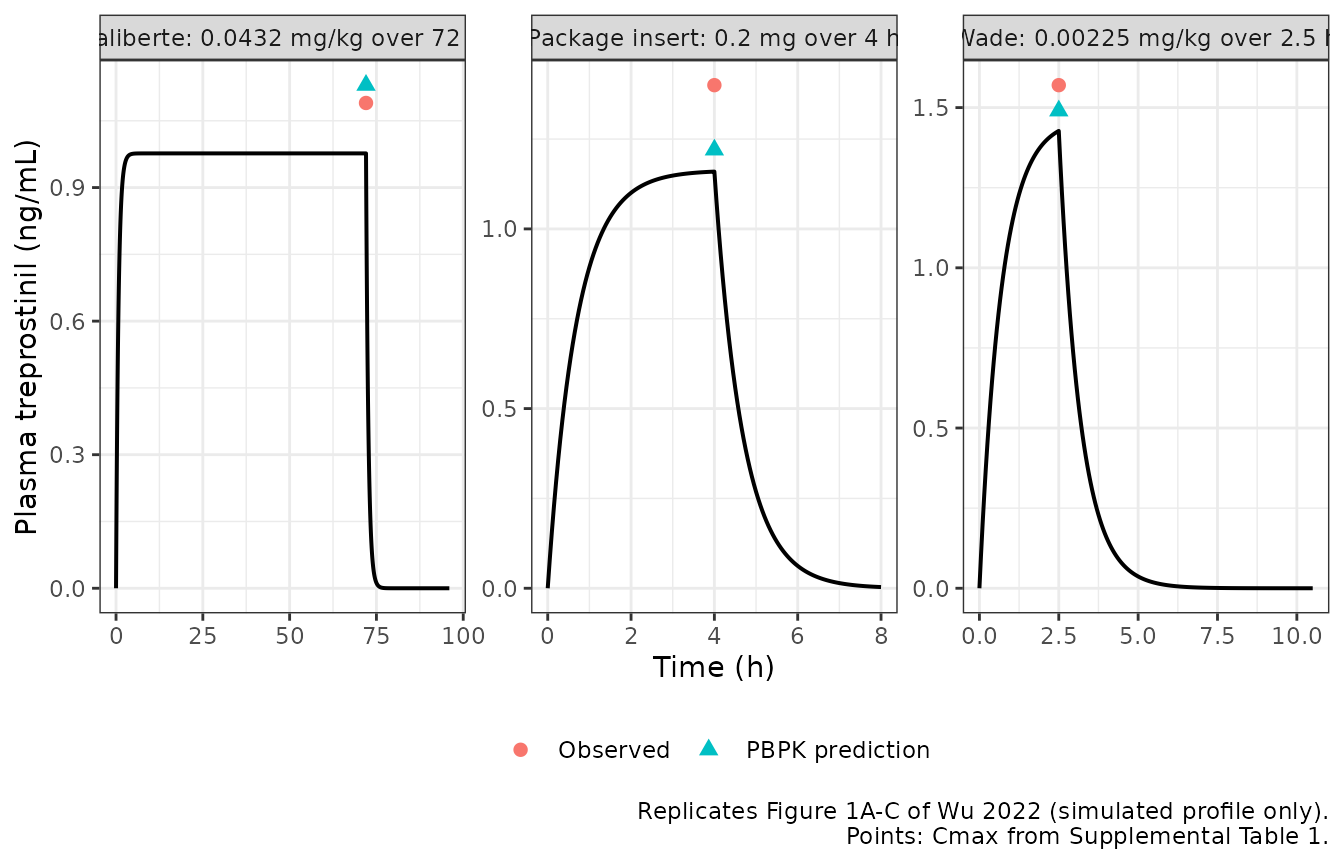

PKNCA validation

Each arm uses its own AUC window, matching Supplemental Table 1: 0-10.5 h, 0-96 h and 0-8 h. A second, open-ended interval feeds the closed-form gates.

# Drop the numerically-zero tail that follows each peak, so the half-life
# fit does not follow integrator noise.
conc <- sim |>
  dplyr::filter(!is.na(Cc)) |>
  dplyr::group_by(id) |>
  dplyr::filter(time <= time[which.max(Cc)] | Cc >= 1e-6 * max(Cc)) |>
  dplyr::ungroup() |>
  dplyr::select(id, time, Cc, arm)

dose_df <- events |>
  dplyr::filter(evid == 1L) |>
  dplyr::select(id, time, amt, arm) |>
  dplyr::left_join(regimens |> dplyr::select(id, dur_h), by = "id")

stopifnot(nrow(conc) > 0, nrow(dose_df) == 3L)

conc_obj <- PKNCA::PKNCAconc(conc, Cc ~ time | arm + id,
                             concu = "ng/mL", timeu = "h")
dose_obj <- PKNCA::PKNCAdose(dose_df, amt ~ time | arm + id,
                             doseu = "mg", route = "intravascular",
                             duration = "dur_h")

intervals <- dplyr::bind_rows(
  regimens |>
    dplyr::transmute(arm, start = 0, end = t_end,
                     cmax = TRUE, tmax = TRUE, auclast = TRUE,
                     aucinf.obs = FALSE, half.life = FALSE),
  regimens |>
    dplyr::transmute(arm, start = 0, end = Inf,
                     cmax = FALSE, tmax = FALSE, auclast = FALSE,
                     aucinf.obs = TRUE, half.life = TRUE)
) |>
  as.data.frame()

nca <- PKNCA::pk.nca(PKNCA::PKNCAdata(conc_obj, dose_obj,
                                      intervals = intervals))

nca_df <- as.data.frame(nca) |>
  dplyr::filter(PPTESTCD %in% c("cmax", "tmax", "auclast",
                                "aucinf.obs", "half.life"))

knitr::kable(
  nca_df |>
    dplyr::mutate(PPORRES = signif(PPORRES, 4)) |>
    dplyr::select(arm, start, end, PPTESTCD, PPORRES),
  caption = "PKNCA results for the three simulated intravenous infusions."
)

PKNCA results for the three simulated intravenous infusions.

arm	start	end	PPTESTCD	PPORRES
Wade: 0.00225 mg/kg over 2.5 h	0	10.5	auclast	3.6620
Wade: 0.00225 mg/kg over 2.5 h	0	10.5	cmax	1.4270
Wade: 0.00225 mg/kg over 2.5 h	0	10.5	tmax	2.5000
Wade: 0.00225 mg/kg over 2.5 h	0	Inf	tmax	2.5000
Wade: 0.00225 mg/kg over 2.5 h	0	Inf	half.life	0.4739
Wade: 0.00225 mg/kg over 2.5 h	0	Inf	aucinf.obs	3.6620
Laliberte: 0.0432 mg/kg over 72 h	0	96.0	auclast	70.3300
Laliberte: 0.0432 mg/kg over 72 h	0	96.0	cmax	0.9767
Laliberte: 0.0432 mg/kg over 72 h	0	96.0	tmax	23.6000
Laliberte: 0.0432 mg/kg over 72 h	0	Inf	tmax	23.6000
Laliberte: 0.0432 mg/kg over 72 h	0	Inf	half.life	0.4739
Laliberte: 0.0432 mg/kg over 72 h	0	Inf	aucinf.obs	70.3300
Package insert: 0.2 mg over 4 h	0	8.0	auclast	4.6490
Package insert: 0.2 mg over 4 h	0	8.0	cmax	1.1590
Package insert: 0.2 mg over 4 h	0	8.0	tmax	4.0000
Package insert: 0.2 mg over 4 h	0	Inf	tmax	4.0000
Package insert: 0.2 mg over 4 h	0	Inf	half.life	0.4739
Package insert: 0.2 mg over 4 h	0	Inf	aucinf.obs	4.6510

Closed-form gates

For a one-compartment model with a constant-rate infusion, AUCinf = dose / CL holds exactly. The terminal half-life after the infusion ends is exactly log(2) * vc / cl. These identities check the NCA setup as much as the model.

get_nca <- function(a, p) {
  v <- nca_df$PPORRES[nca_df$arm == a & nca_df$PPTESTCD == p]
  if (length(v) != 1L) stop("no unique NCA row for '", a, "' / ", p)
  v
}

vc_mod <- exp(theta[["lvc"]])
cl_mod <- exp(theta[["lcl_renal"]]) + exp(theta[["lcl_nonren"]])

gate <- regimens |>
  dplyr::rowwise() |>
  dplyr::mutate(
    aucinf_nca    = get_nca(arm, "aucinf.obs"),
    aucinf_closed = dose_mg / cl_mod * 1000,
    auc_pct       = 100 * (aucinf_nca - aucinf_closed) / aucinf_closed,
    thalf_nca     = get_nca(arm, "half.life"),
    thalf_closed  = log(2) * vc_mod / cl_mod,
    thalf_pct     = 100 * (thalf_nca - thalf_closed) / thalf_closed
  ) |>
  dplyr::ungroup()

knitr::kable(
  gate |>
    dplyr::select(arm, aucinf_nca, aucinf_closed, auc_pct,
                  thalf_nca, thalf_closed, thalf_pct) |>
    dplyr::mutate(dplyr::across(where(is.numeric), \(x) signif(x, 5))),
  caption = "NCA output vs. the closed-form one-compartment identities."
)

NCA output vs. the closed-form one-compartment identities.

arm	aucinf_nca	aucinf_closed	auc_pct	thalf_nca	thalf_closed	thalf_pct
Wade: 0.00225 mg/kg over 2.5 h	3.6624	3.6628	-0.0118720	0.47392	0.47392	0
Laliberte: 0.0432 mg/kg over 72 h	70.3250	70.3260	-0.0004232	0.47392	0.47392	0
Package insert: 0.2 mg over 4 h	4.6508	4.6512	-0.0075950	0.47392	0.47392	0

# Both identities are exact for this model; what remains is trapezoidal
# error on the 0.05 h grid and ODE integration error. Bounds sit well above
# the achieved agreement but far below any parameter-level mistake (a wrong
# volume or clearance moves these by tens of percent).
stopifnot(nrow(gate) == 3L,
          max(abs(gate$auc_pct))   < 0.5,
          max(abs(gate$thalf_pct)) < 0.5)
cat(sprintf(paste("AUCinf reproduces dose/CL to within %.3f%% and the terminal",
                  "half-life (%.3f h) reproduces log(2)*vc/cl to within %.3f%%",
                  "across all %d arms.\n"),
            max(abs(gate$auc_pct)), gate$thalf_closed[1],
            max(abs(gate$thalf_pct)), nrow(gate)))
#> AUCinf reproduces dose/CL to within 0.012% and the terminal half-life (0.474 h) reproduces log(2)*vc/cl to within 0.000% across all 3 arms.

Comparison against the published NCA

Against the paper’s own PBPK predictions

This comparison decides whether the reduction is faithful to the platform model. Supplemental Table 1 reports the PBPK model’s predicted Cmax and AUC over each study’s window. Nothing was tuned to reach them.

nca_window <- nca_df |>
  dplyr::filter(PPTESTCD %in% c("cmax", "auclast"), is.finite(end))

published_pred <- tibble::tribble(
  ~arm,                                  ~cmax, ~auclast,
  "Wade: 0.00225 mg/kg over 2.5 h",       1.49,     4.07,
  "Laliberte: 0.0432 mg/kg over 72 h",    1.13,    81.10,
  "Package insert: 0.2 mg over 4 h",      1.22,     4.98
)

cmp_pred <- nlmixr2lib::ncaComparisonTable(
  simulated = nca_window,
  reference = published_pred,
  by        = "arm",
  units     = c(cmax = "ng/mL", auclast = "ng*h/mL"),
  tolerance_pct = 20
)

knitr::kable(
  cmp_pred,
  caption = paste("Reduction vs. the Simcyp predictions in Wu 2022",
                  "Supplemental Table 1 (AUC over 0-10.5, 0-96 and 0-8 h).",
                  "* differs by >20%."),
  align = c("l", "l", "r", "r", "r")
)

Reduction vs. the Simcyp predictions in Wu 2022 Supplemental Table 1 (AUC over 0-10.5, 0-96 and 0-8 h). * differs by >20%.

NCA parameter	arm	Reference	Simulated	% diff
Cmax (ng/mL)	Wade: 0.00225 mg/kg over 2.5 h	1.49	1.43	-4.2%
Cmax (ng/mL)	Laliberte: 0.0432 mg/kg over 72 h	1.13	0.977	-13.6%
Cmax (ng/mL)	Package insert: 0.2 mg over 4 h	1.22	1.16	-5.0%
AUClast (ng*h/mL)	Wade: 0.00225 mg/kg over 2.5 h	4.07	3.66	-10.0%
AUClast (ng*h/mL)	Laliberte: 0.0432 mg/kg over 72 h	81.1	70.3	-13.3%
AUClast (ng*h/mL)	Package insert: 0.2 mg over 4 h	4.98	4.65	-6.7%

# `% diff` is formatted as text (a trailing "*" marks rows over tolerance),
# so strip the formatting before testing. The solve is deterministic, so
# this bound does not have to absorb any cohort sampling noise.
pct_pred <- suppressWarnings(
  as.numeric(gsub("[^0-9.eE+-]", "", as.character(cmp_pred[["% diff"]])))
)
stopifnot(sum(is.finite(pct_pred)) == 6L,
          max(abs(pct_pred), na.rm = TRUE) < 15)
cat(sprintf(paste("All %d comparisons against the PBPK predictions agree",
                  "within 15%%; largest discrepancy %.1f%%.\n"),
            sum(is.finite(pct_pred)), max(abs(pct_pred), na.rm = TRUE)))
#> All 6 comparisons against the PBPK predictions agree within 15%; largest discrepancy 13.6%.

How to read the table:

• The two short infusions are the sharpest test because their per-kilogram (Wade) or flat (package insert) dose is close to steady state by the end of the infusion. Cmax agrees to within about 5% for both.
• Every AUC runs low, by 7-13%. Part of the gap is that the platform’s simulated clearance runs slightly below its own 43 L/h input. Supplemental Table 1 reports the simulated mean clearance as 40.9, 40.1 and 41.7 L/h for the three studies. The reduction uses the 43 L/h that section 2.2 gives as the model input, and does not adopt the platform’s simulated output. The flat-dose package-insert arm isolates this effect, because neither its dose nor its AUC depends on body weight. There, the PBPK prediction implies 0.2 mg / 4.98 ng*h/mL = 40.2 L/h, and the ratio 40.2 / 43 accounts for the whole -6.6% gap (gate below). The two per-kilogram arms add a body-weight effect on top of it.
• The Laliberte 72 h infusion carries the largest gap, -14% on Cmax. Its Cmax is the steady state dose rate / CL, and the dose rate scales with body weight, so this arm is the most sensitive to the 70 kg assumption (next section).

# Package insert: flat 0.2 mg dose, so the AUC ratio is weight-free and
# must equal the ratio of the platform's implied clearance to the 43 L/h input.
auc_pi     <- nca_window$PPORRES[nca_window$arm == "Package insert: 0.2 mg over 4 h" &
                                   nca_window$PPTESTCD == "auclast"]
cl_pbpk_pi <- 0.2 / 4.98 * 1000          # L/h implied by Supplemental Table 1
stopifnot(abs((auc_pi / 4.98) / (cl_pbpk_pi / cl_mod) - 1) < 0.005)
cat(sprintf(paste("Package insert: AUC ratio %.4f vs clearance ratio %.4f",
                  "(PBPK-implied %.2f L/h / input %.0f L/h).\n"),
            auc_pi / 4.98, cl_pbpk_pi / cl_mod, cl_pbpk_pi, cl_mod))
#> Package insert: AUC ratio 0.9334 vs clearance ratio 0.9340 (PBPK-implied 40.16 L/h / input 43 L/h).

Against the observed data

The same table also reports the observed values for each study. These are shown for completeness; they test the platform model as much as the reduction.

published_obs <- tibble::tribble(
  ~arm,                                  ~cmax, ~auclast,
  "Wade: 0.00225 mg/kg over 2.5 h",       1.57,     3.49,
  "Laliberte: 0.0432 mg/kg over 72 h",    1.09,    77.26,
  "Package insert: 0.2 mg over 4 h",      1.40,     4.11
)

cmp_obs <- nlmixr2lib::ncaComparisonTable(
  simulated = nca_window,
  reference = published_obs,
  by        = "arm",
  units     = c(cmax = "ng/mL", auclast = "ng*h/mL"),
  tolerance_pct = 20
)

knitr::kable(
  cmp_obs,
  caption = paste("Reduction vs. observed values in Wu 2022 Supplemental",
                  "Table 1. * differs by >20%."),
  align = c("l", "l", "r", "r", "r")
)

Reduction vs. observed values in Wu 2022 Supplemental Table 1. * differs by >20%.

NCA parameter	arm	Reference	Simulated	% diff
Cmax (ng/mL)	Wade: 0.00225 mg/kg over 2.5 h	1.57	1.43	-9.1%
Cmax (ng/mL)	Laliberte: 0.0432 mg/kg over 72 h	1.09	0.977	-10.4%
Cmax (ng/mL)	Package insert: 0.2 mg over 4 h	1.4	1.16	-17.2%
AUClast (ng*h/mL)	Wade: 0.00225 mg/kg over 2.5 h	3.49	3.66	+4.9%
AUClast (ng*h/mL)	Laliberte: 0.0432 mg/kg over 72 h	77.3	70.3	-9.0%
AUClast (ng*h/mL)	Package insert: 0.2 mg over 4 h	4.11	4.65	+13.1%

pct_obs <- suppressWarnings(
  as.numeric(gsub("[^0-9.eE+-]", "", as.character(cmp_obs[["% diff"]])))
)
stopifnot(sum(is.finite(pct_obs)) == 6L,
          max(abs(pct_obs), na.rm = TRUE) < 25)

The paper’s acceptance criterion is a prediction error within 50% (section 2.5), and the reduction stays within 20% of every observed value. Package-insert Cmax is the largest miss, at -17%. The Simcyp model itself also under-predicts that value (1.22 against 1.40 ng/mL).

Sensitivity to the unreported body weight

Body weight enters twice: in the volume (0.42 L/kg) and in the two per-kilogram doses. Clearance is an absolute 43 L/h. The table below gives the closed-form Cmax and AUC over each window for reference weights of 70, 75 and 80 kg, as percent differences from the PBPK predictions. Nothing here is fed back into the model.

inf_closed <- function(dose_mg, dur_h, t_end, wt) {
  vc <- 0.42 * wt
  k  <- cl_mod / vc
  r  <- dose_mg / dur_h
  cmax <- r / cl_mod * (1 - exp(-k * dur_h)) * 1000
  # AUC over [0, t_end]: infusion phase plus the post-infusion decay.
  auc_inf_phase <- r / cl_mod * (dur_h - (1 - exp(-k * dur_h)) / k)
  auc_post      <- cmax / 1000 / k * (1 - exp(-k * (t_end - dur_h)))
  c(cmax = cmax, auclast = (auc_inf_phase + auc_post) * 1000)
}

wt_sens <- tidyr::crossing(regimens |> dplyr::select(arm, dur_h, t_end),
                           wt = c(70, 75, 80)) |>
  dplyr::mutate(
    dose_mg = dplyr::case_when(
      grepl("Wade", arm)      ~ 0.00225 * wt,
      grepl("Laliberte", arm) ~ 0.0432 * wt,
      TRUE                    ~ 0.2
    )
  ) |>
  dplyr::rowwise() |>
  dplyr::mutate(
    cmax    = inf_closed(dose_mg, dur_h, t_end, wt)[["cmax"]],
    auclast = inf_closed(dose_mg, dur_h, t_end, wt)[["auclast"]]
  ) |>
  dplyr::ungroup() |>
  dplyr::left_join(published_pred |>
                     dplyr::rename(cmax_pbpk = cmax, auc_pbpk = auclast),
                   by = "arm") |>
  dplyr::mutate(cmax_pct = 100 * (cmax / cmax_pbpk - 1),
                auc_pct  = 100 * (auclast / auc_pbpk - 1))

# The closed form at 70 kg must match the simulated NCA (cross-check).
chk70 <- wt_sens |> dplyr::filter(wt == 70) |>
  dplyr::left_join(nca_window |> dplyr::filter(PPTESTCD == "cmax") |>
                     dplyr::select(arm, cmax_sim = PPORRES), by = "arm")
stopifnot(max(abs(chk70$cmax / chk70$cmax_sim - 1)) < 1e-3)

knitr::kable(
  wt_sens |>
    dplyr::select(arm, wt, cmax_pct, auc_pct) |>
    dplyr::mutate(dplyr::across(c(cmax_pct, auc_pct), \(x) round(x, 1))) |>
    dplyr::rename("Body weight (kg)"         = wt,
                  "Cmax vs PBPK (% diff)"    = cmax_pct,
                  "AUC vs PBPK (% diff)"     = auc_pct),
  caption = "Closed-form sensitivity of the comparison to the reference weight."
)

Closed-form sensitivity of the comparison to the reference weight.

arm	Body weight (kg)	Cmax vs PBPK (% diff)	AUC vs PBPK (% diff)
Laliberte: 0.0432 mg/kg over 72 h	70	-13.6	-13.3
Laliberte: 0.0432 mg/kg over 72 h	75	-7.4	-7.1
Laliberte: 0.0432 mg/kg over 72 h	80	-1.2	-0.9
Package insert: 0.2 mg over 4 h	70	-5.0	-6.6
Package insert: 0.2 mg over 4 h	75	-5.1	-6.7
Package insert: 0.2 mg over 4 h	80	-5.3	-6.7
Wade: 0.00225 mg/kg over 2.5 h	70	-4.2	-10.0
Wade: 0.00225 mg/kg over 2.5 h	75	1.9	-3.6
Wade: 0.00225 mg/kg over 2.5 h	80	7.8	2.9

The Laliberte arm moves the most, because both its dose rate and its volume scale with weight. A heavier reference weight closes most of that gap. The package-insert arm used a flat dose and does not move. No weight is printed, so 70 kg is kept as the standing rounded standard. The table shows how much the comparison depends on that choice, and that no plausible adult weight changes the conclusion.

Assumptions and deviations

1. Body weight of 70 kg is assumed. Table 3 states the volume in L/kg, and two of the three intravenous studies dosed per kilogram. No body weight appears anywhere in the paper or its supplement; Table 1 gives only race, sex split and age range. The 70 kg reference is the standing rounded-standard convention, and it is the only value in the model that does not come from the source. WT is recorded in covariatesDataExcluded rather than carried as a live covariate. The clearance is an absolute 43 L/h, and its weight scaling lives in the unpublished Simcyp population file, so scaling volume alone would make the model internally inconsistent.
2. The oral arm was deliberately not reduced. As shown above, the printed fa * Fg * Fh = 0.25 with the intravenous clearance gives an AUC 48% above the platform’s own prediction for any absorption shape. The printed Fh of 0.60 would need a hepatic blood flow of about 180 L/h. The oral model’s systemic clearance (after the fraction unbound was changed to 0.04) and its ADAM absorption layer are platform-database outputs that the paper does not print. The extended-release tablet studies, the hepatic-impairment extrapolation (predicted AUC 2.4-, 3.8- and 4.6-fold healthy for Child-Pugh A, B and C) and the patient extrapolations are therefore out of scope.
3. The reduction is mono-exponential. The source is a full-PBPK model, and only a lumped Vss is reported, so no distribution phase can be reconstructed. Treprostinil’s tissue Kp values are all low (0.05-0.22, except adipose at 1.20), and the volume is small (0.42 L/kg). The cost is modest here: the reduction is within 14% of every PBPK-predicted Cmax and AUC.
4. The clearance is the input, not the platform’s output. Section 2.2 gives 43 L/h as the average intravenous clearance of references 4, 10 and 11, and the retrograde model back-calculated the enzyme intrinsic clearances from it. The Simcyp simulations return a slightly lower mean clearance (40.1-41.7 L/h in Supplemental Table 1). That accounts for all of the package-insert AUC gap and part of the other two. The printed input is used rather than adopting the simulated output, which would amount to tuning toward the answer key.
5. The volume is the final model’s predicted Vss. Table 3 gives 0.42 L/kg predicted and 0.40 L/kg observed. The predicted value is the one produced by the optimized Kp scalar and adipose Kp, so it describes the final model. The per-study simulated Vss values in Supplemental Table 1 (0.65, 0.43 and 0.46 L/kg) are NCA estimates over truncated windows and are not used.
6. No inter-individual variability and no residual error. Wu 2022 is a PBPK simulation study, not a population-PK fit. Its 5th-95th percentile bands are the spread of a Simcyp virtual population driven by unpublished population files, not estimated variance components. Rather than invent variances, the model has no etas and propSd is fixed at zero, so it is a deterministic typical-value simulator.
7. Elimination-route fractions are not encoded separately. The CYP2C8 and CYP2C9 split (90:10 of metabolism; predicted 81% CYP2C8 contribution overall), the biliary arm and the additional systemic clearance do not change the plasma profile. They are recorded in population$notes and lumped in lcl_nonren. Only the renal arm is separate, because Table 4 prints it as a clearance.
8. The lung prediction is not encoded. The paper’s statement that lung exposure is about 0.17 times plasma is the Rodgers and Rowland lung Kp (Table 3). It is a steady-state tissue:plasma ratio inside the platform’s lung compartment, not an output of this reduction. Users who want the paper’s estimate can multiply Cc by 0.17.
9. No errata were found. A EuropePMC search on 2026-10-02 found no correction notice for doi:10.1111/bcp.14966.